In the last section, we discussed the creation of 3D breaklines for enforcing situations where the elevation must be a constant along the breakline. The most common example of this application is “water body flattening” such as lakes and ponds. In this final section we will consider the case of varying elevation along the breakline.
Recall that, for our purposes, a 3D breakline is a vector (feature) that has an elevation value (Z) associated with each vertex. Generally, 3D breaklines can be divided into two categories – those with the same elevation for each vertex (used for flat water bodies, for example) and those with the ability to store a different elevation value for each vertex (a down-stream flow polyline, for example).
In this section, let’s look at a varying Z example such as the edges of a road or a downstream flow. As with flat water bodies, a common method of collecting breaklines is to use heads-up digitizing from an orthophoto for the X, Y (planimetric) aspects of the construction and to probe the LIDAR (or, more generally, point cloud data) for the Z value. Unlike the constant Z flat water body breaklines, we must store the Z for varying elevation breaklines at each vertex. This means that these breaklines are always represented by 3D features.
One very useful way to locate and visualize drainage is via a contour display. Figure 28 shows an area of drainage. I have filtered the point cloud to ground points only and visualized as a triangulated irregular network (TIN). The area of drainage has been roughly sketched in blue using LP360 Feature Edit tools. Note that the contours “point” upstream due to the depression formed by the drainage. Thus you can use the ground class along with an examination of LP360’s dynamic contours to identify drainage location and direction.
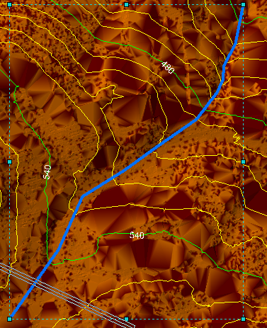
Figure 28: Visualizing Drainage via Contours
There are at least two approaches to digitizing the actual drainage breakline. The first is to identify the drainage purely from a two-dimensional top view (“map view”). After digitizing, the Z value can be obtained from the point cloud surface via automatic probing. In LP360 we call this process of probing the point cloud data for the elevation value “Z Conflation.” The problem with this approach is that, even with contours, it can be difficult to correctly identify the lowest point of drainage in the planimetric sense. More importantly is enforcing a hydrological model. We need to ensure that drainage is strictly monotonically decreasing as we move downstream from vertex to vertex. Fortunately, LP360 contains advanced tools for properly enforcing downstream constraints.
Figure 29 depicts the dialogs in LP360 for digitizing a downstream constraint. The dialog to the left contains overall “Z conflation” settings where general parameters are configured. Note that I have set the “Conflation Method” to “Downstream Constraint.”
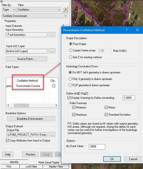
Figure 29: The Downstream Constraint Tool in LP360
The dialog to the right in Figure 29 is used for configuring the specifics of the conflation method; in this case, the downstream constraint. All conflation methods in LP360 allow you to change the vertex spacing, if desired. The general choices are:
- Pure Drape – This creates a vertex at each point where the breakline intersects the edge of the triangulated irregular network (TIN) created from the point cloud
- Create vertex every X map units – inserts new vertices at the user specified spacing
- Get Z for existing vertices – do not modify the existing vertex locations.
There is a tool in LP360 called Respace Vertices that will allow you to achieve any vertex spacing desired should you find that your conflated features do not meet your vertex spacing needs.
The remainder of the setting of the dialog on the right in Figure 29 are related to error monitoring. The downstream constraint will, after the vector digitizing is complete, adjust the assigned values such that the monotonicity is maintained (that is, each subsequent vertex as one walks down the breakline has a Z value lower than or equal to the immediately previous vertex).
Most topology systems use the sense (direction) of a feature/vector to determine the downstream direction. Usually, moving in the direction of increasing vertex ID is considered the downstream direction. The first section of the error management of the downstream constraint dialog provides some self-evident options for how this is handled. For example, the system can automatically flip the direction of a downstream feature if you inadvertently draw uphill.
The second section of the error portion of the dialog allows you to monitor how much a particular vertex is moved by the system to maintain the monotonic constraint. The distance between the surface derived from the point cloud and the Z of the vertex is referred to as the “Delta.” We take this measure to be the Adjusted Z (the final vertex Z) minus the surface (or original) Z. Thus an adjustment of a vertex beneath the surface creates a negative Delta. If desired, the Delta of every vertex can be stored in the Measure (M) value of the vertex, assuming you created a 3D polyline feature layer with M values.
I think creating M values is a very good way to validate the downstream features that you collect. You can use Feature Analyst to very quickly test all your downstream features against a quality assessment criterion. For example, in the settings of Figure 30, I want to find all vertices that are over ¼ foot above or below the point cloud surface. Once you have performed all the quality testing, you can easily remove M values from the feature file by doing a Create Feature from Feature command with the target layer being a 3D polyline layer without M values.
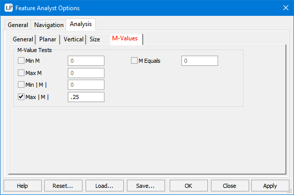
Figure 30: Testing M Values of a feature
Finally (going back to Figure 29), summary statistics for each feature can be stored in the Attribute table. The computed values include:
• Minimum – The largest delta below the TIN surface
• Maximum – The largest delta above the TIN surface
• Mean – The mean of the deltas
• Standard deviation – the statistical standard deviation of all the deltas of the vector
The actual digitizing of a breakline in LP360 is performed using both the Map View and the Profile View. The Map View provides the planimetric location whereas the Profile View allows you to visualize the vertical placement.
A general technique that I find useful for drainage centerline is to turn on contour display in the Map View and identify the drainage that I want to digitize using the drainage induced distortions in the contours. It can be useful to roughly digitize these locations using the Feature Edit tools in LP360. I then set up for digitizing in the Profile/Map View. This generally is initiated by beginning a breakline sketch in the Map View; the Profile View will be automatically synchronized while drawing. This is depicted in Figure 31. Note the red box in the Profile View. Here I have boxed in the intersection of the projection from the Map View (vertical white line) with the Ground Points (orange in the Profile View of Figure 31). This vertical line is “dropped” from the Map View into the Profile View and tracks the cursor as you adjust the position in the Map View. Thus one would adjust the location of the vertex of the breakline by moving to a point such that the dropped line crosses the surface model at the lowest point.
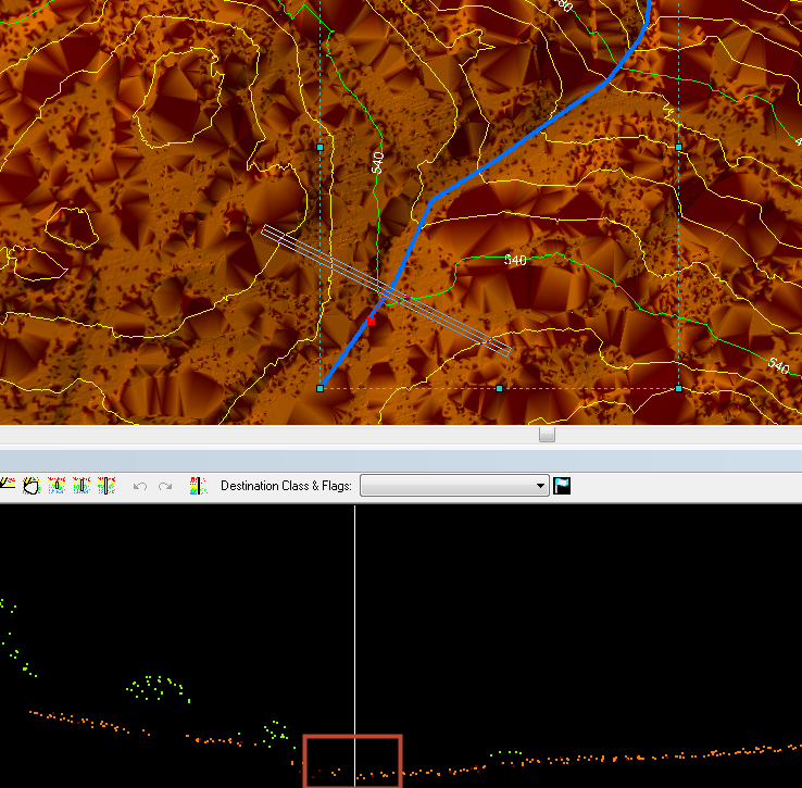
Figure 31: Digitizing a breakline using the profile view
The downstream constraint algorithm in LP360 constrains the breakline to three criteria:
• The polyline must be monotonically decreasing as one moves in the downstream direction. Note that vertex n+1 can have the same elevation as vertex n but it cannot be lower. Therefore, level stretches are OK.
• The initial and final vertices are “anchors” and will not be moved. This means the algorithm will fail if the final vertex is higher than the initial vertex.
• The intermediate vertices are adjusted to meet the first criterion such that the distance, in Z, from the vertex to the surface points is minimized.
LP360 can do “on-the-fly” conflation; that is, the vertices are adjusted as each is digitized. For downstream constraint, I recommend using a surface conflation task (surface or lowest point) and then applying the downstream constraint as a second step in the process.
Using this method, the breakline being digitized is depicted in Figure 32 as the white line with vertices as colored boxes. In the profile view, note the vertex in cyan. This vertex can be moved horizontally by dragging the vertex icon in the Profile View to the right or left. This makes for quick editing to place the vertex right over your estimation of the thalweg (slightly to the left in the Profile View of Figure 32). Notice that I am using the shape of the dynamic contours in the Map View as clues as to the proper location of the thalweg.
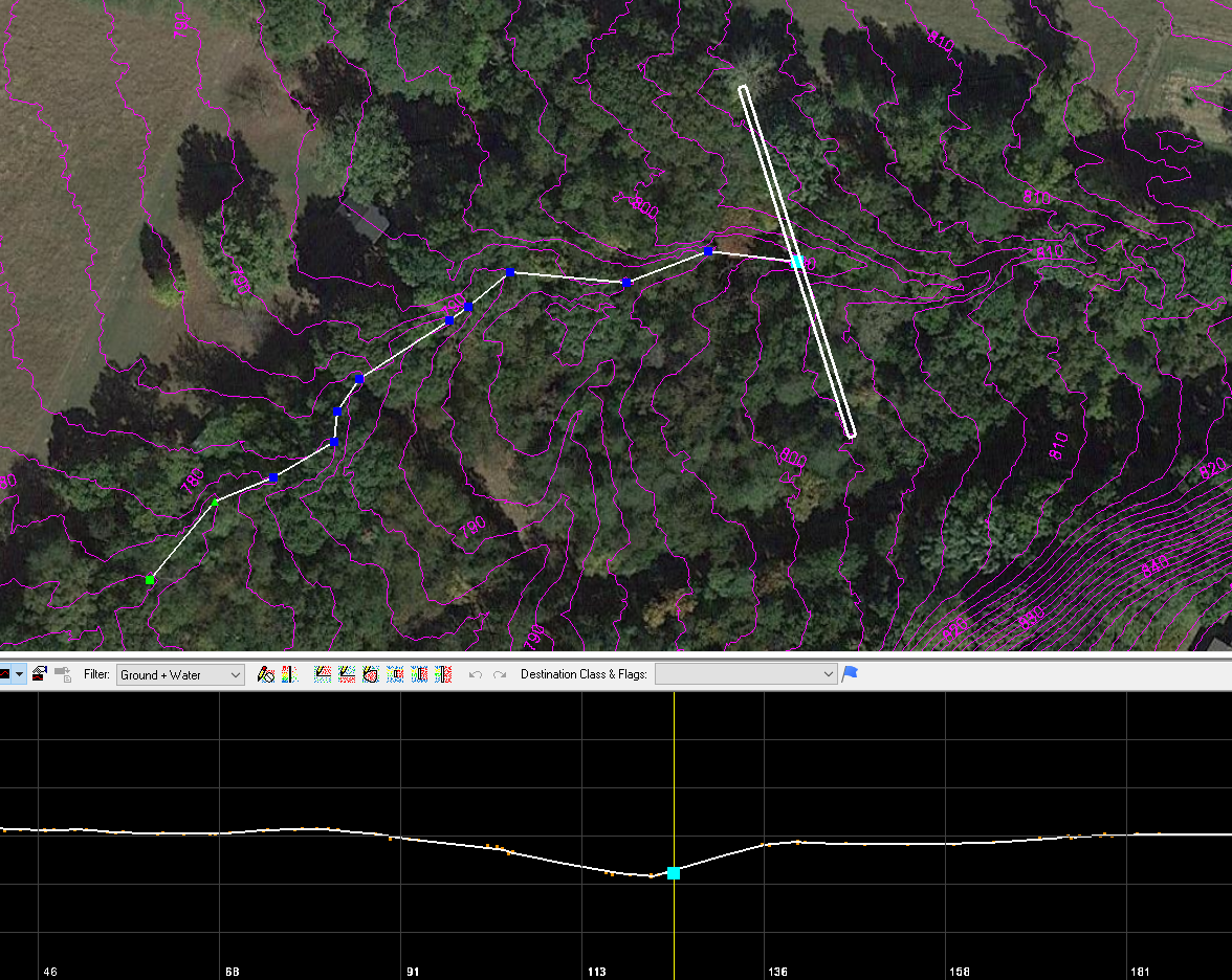
Figure 32: The digitized breakline (white)
In Figure 33 is depicted the stream feature prior to downstream constraint. I have used Feature Analyst to examine this feature. It indicates that the feature is violating the downstream constraint and, furthermore, this violation is occurring at vertex 13. As you can see, Feature Analyst is a very powerful tool!
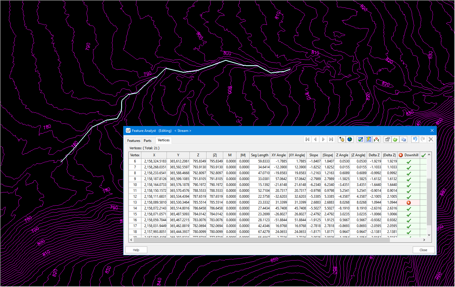
Figure 33: Downstream feature prior to constraint
I next apply the downstream constraint PCT that we previously constructed. This can be done by changing the Auto Z tool in the Feature Edit toolbar or simply running the downstream PCT directly on the feature.
Finally, in Figure 34 is depicted the enforced downstream constraint breakline (the blue vector). Note that the effect of a downstream constraint on the contours will be quite subtle if the thalweg line is drawn in the correction location. This is because the point cloud itself is a very accurate representation of the drainage topography and hence, you would not expect a significant change. Note that I have selected the downstream feature and displayed its vertices in Feature Analyst. The feature passes the “Downstream” test. I also added a test for maximum M value. Recall that we set the M values to record the distance the feature vertex had to be moved above or below the LIDAR surface to maintain monotonicity. I set my test to alert me if the deviation exceeded 0.25 feet. You can see the offending vertices highlighted in the table with a red X icon under the “Max Absolute M Value” test. I can immediately drive to each of these suspect vertices by clicking the row in the Feature Analyst vertex table.
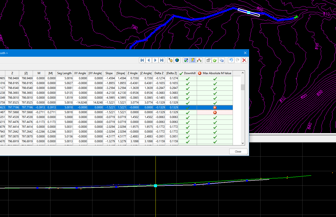
Figure 34: The enforced downstream constraint
We support several other variable Z breaklines in LP360. Among these are:
- Double line drains (“river flattening”) – This is used for wider streams and rivers where the overall elevation in the direction of flow is monotonically decreasing so the banks perpendicular to the direction of flow must be at the same elevation (otherwise the flow direction would be cross channel rather than down channel).
- Retaining Wall – The retaining wall tool allows you to digitize parallel lines with a slight displacement. Each line can be conflated using a different algorithm. The primary use is along walls where using the high points for one line and the low points for the parallel line will create a model of the wall. This model can be used in subsequent breakline enforcements.
This concludes the discussion on breakline collection and enforcement within the LP360 product. As you can see, this is a very rich area of LP360 and a reason that LP360 is one of the most widely used tools in the point cloud industry for adding and visualizing hydrological (and other forms) of constraints. I encourage you to thoroughly review our help files and tutorials if your work involves breakline collection. The tool you need is most likely in our collection!
