Prolog:
I am writing a new whitepaper on model constraints in LP360 (any reference to LP360 where I do not add the term “for ArcGIS,” I am talking about the standalone version. This document is extracted and heavily revised from a series of articles that I wrote for the GeoCue Group Newsletter in 2013. The big change is that, at that time, we only had enforcement in the standalone version of LP360. Even in LP360 for ArcGIS, one had to use a number of ArcGIS tools to fully edit a breakline model. Now, we are essentially feature-complete with new tools in standalone LP360. Not only are all of the breakline creation tools present, but we also have a very rich set of 3D feature edit tools. Finally, you can do very high-performance 3D breakline creation and editing in a standalone Windows 64-bit application.
For the next perhaps 5 issues of GeoCue Group News, I will present these new tools. While this series is aimed squarely at our product, LP360, the information on constraining point cloud models is general to any software implementation. Even if you are not a user of our LP360 software, you will still gain a pretty good understanding of how breaklines are used to modify three-dimensional (3D) model data.
1 Introduction
One of the more powerful capabilities within LP360 is breakline capture and enforcement. In fact, many LIDAR production shops use LP360 as their tool of choice for supplementing point cloud data derived from LIDAR or correlated imagery (so-called Structure from Motion, SfM, Dense Image Matching, DIM, Semi-Global Matching, SGM and a few other monikers) with breaklines. But what are breaklines and how should they be used? In this paper, I will be providing some background information on elevation modeling and then delve in to how these advanced features are implemented in our LP360 (native 64-bit Windows version) tools.
2 Why Constrain Models?
The first thing to do is motivate this topic. What is a breakline and why are they needed?
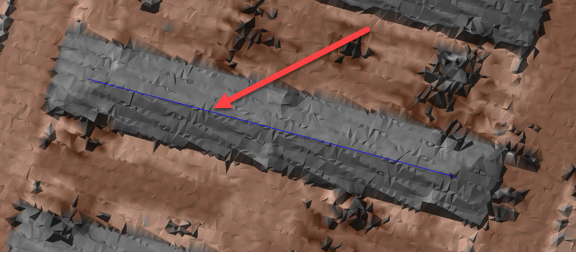
When we collect data from the real world using a LIDAR sensor or 3D points derived from imagery (“photogrammetry”), we are sampling the real world. Our sample points are sparse compared to the essentially continuous data that are being sampled. For example, if we are sampling an area of bare earth with no holes in the ground, the earth is continuous. However, our sample points will have some spacing between them. This means the fidelity of the model is not as high as that of the data that are being sampled. The coarser the sample spacing, the lower the fidelity. An example of a roof line is shown in Figure 1. We know the roof should show a sharp, well-defined ridge line (I have drawn a blue vector along the ridge). Instead, we see divots where we do not have sufficient points to define the edge.
Figure 1: Divots in a roof line due to low sampling density
If we have a priori knowledge about the data we are sampling, the model rendition can be improved by supplementing the sample data with point, line and polygon features. For example, if we draw in a ridge line for the building in Figure 1 and incorporate that line into the model, the defective ridge line can be repaired.
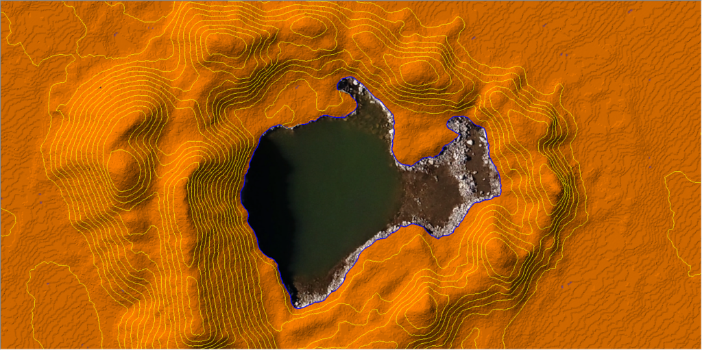
Our a priori knowledge does not have to be exact feature knowledge (that is, I know I should have a linear feature in my data of such and such length with a particular height). In fact, it is usually the case the I know characteristics or constraints rather than specific feature information. For example, I know that a stationary water body such as a non-flowing lake is flat. I am not necessarily given the shore line or the elevation. But still, I can digitize a shore line using heads-up digitizing over an orthophoto, discern the proper water elevation from LIDAR points at the water’s edge and set the shoreline feature Z values all to this same observed value. I can then insert this elevation constraint as a water body flattening polygon in my elevation model. An example of this is shown in Figure 2. Notice that none of the contour lines cross the water body boundary. Of course, a model constraint is not just a constant boundary. We may know other information such as the fact that water, in a gravity flow model, flows only downhill. Thus, we might have a monotonicity enforcement (“downstream constraint”) rule.
Figure 2: Enforcing a water body flattening polygon
There are many uses for breaklines (model constraints) when modeling data. A few examples include:
- Edge definition such as “edge of pavement” for roads, building footprints, edge of streams
- Shorelines of water flat bodies
- Talweg (also thalweg, the channel center) definition for streams
- Edge of bank of a flowing river or stream (a “double line drain”)
- Zero slope centerline of roads (the crown)
- Edges of highwalls in mining
- Stockpile base definition (the stockpile “toe”)
- Ground survey points in areas where the sampling system (for example, photogrammetric modeling) did not penetrate through vegetation to the ground
With the proper point cloud tools (e.g. LP360!), these features can be added to the model. When a derived model is then created (such as generating a raster digital elevation model, DEM), these supplemental breaklines will be enforced during model creation to correct the model deficiencies.
3 The Triangulated Irregular Network
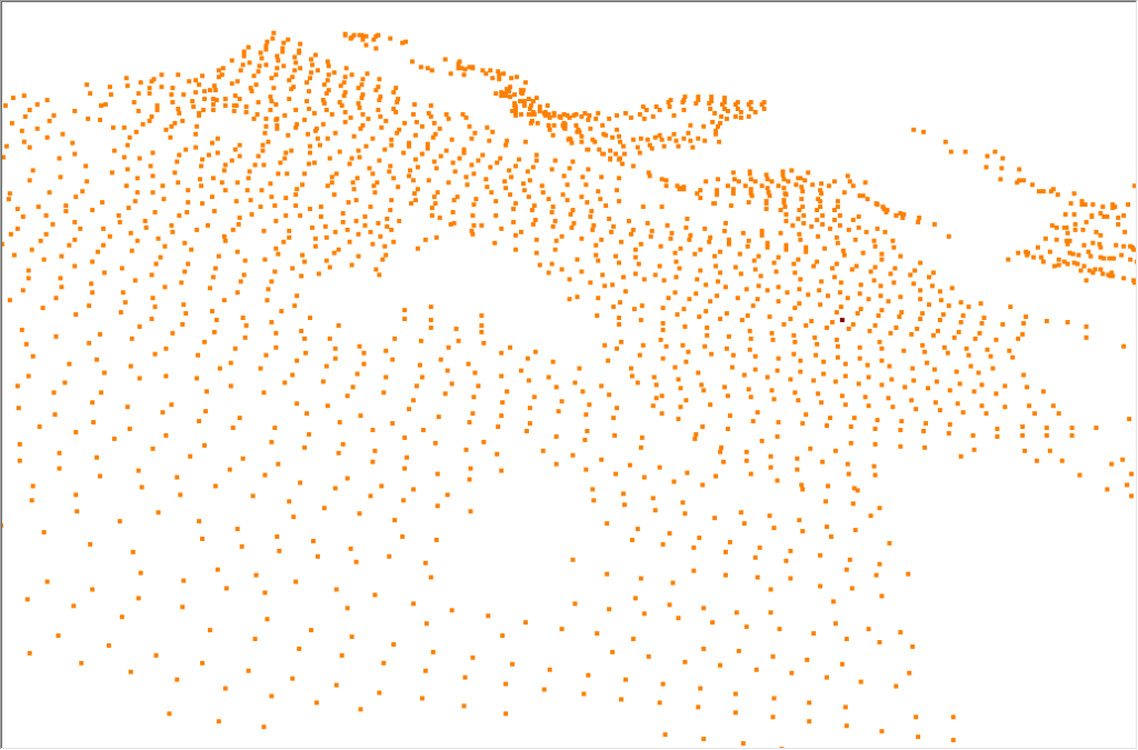
The most common model used for point cloud data is a Triangulated Irregular Network (TIN) derived from the 3D points of the cloud. A portion of a point cloud (in this example, ground points) is illustrated in Figure 3.
Figure 3: A point cloud
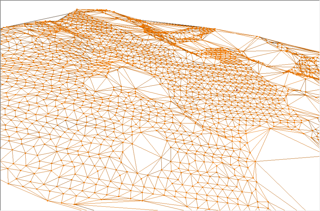
An example of a triangle model of this same project area is illustrated in Figure 4.
Figure 4: The points of Figure 3 rendered as a wireframe TIN
A point cloud comprises discrete 3D points (sampled from a laser scanner or derived by stereo extraction from overlapping images[1]) with voids in between the points. To visualize the point cloud as a surface, we need to “fill in” the space between the points. One of the most common ways of doing this in a Geospatial Information System (GIS) is to connect each point in a triangle mesh (see Figure 4). We create this mesh in a very special way such as to maximize the interior angles of all the triangles (this is the ubiquitous “Delaunay” triangulation technique[2]). This is done because long, skinny triangles tend to cause problems when deriving information from the model.
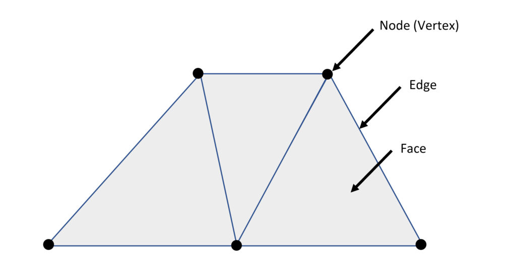
The three important elements of a TIN are:
- Node (vertex) – The points used to construct the TIN
- Edge – The line segment that connects two nodes
- Facet or Face – the triangle formed by three edges
These components are shown in Figure 5.
_______________________________________
[1] Boris Delaunay, circa 1934
[2] Again, commonly called Structure from Motion, SfM, data
Figure 5: Components of the TIN
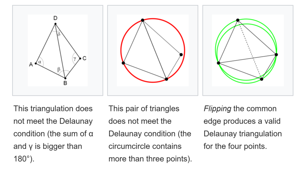
The Delaunay process is depicted in Figure 6 (borrowed from Wikipedia). It is interesting to note that applying the Delaunay criteria to a mesh of triangles can cause a number of edge flips. Edge flipping actually changes the characteristic of the surface model since it moves the “bends” in the model (bends occur at triangle edges). This can be corrected, if need be, by inserting “breaklines” between nodes where the edge needs to be placed. This is discussed in the next section.
Figure 6: Forcing triangles to meet the Delaunay criteria
Thus, we have formed a (T)riangulated (comprising triangles), (I)rregular (the triangles are, in general, different sizes and contain differing angles), (N)etwork (we can traverse the entire mesh by following edges).
When the faces are “filled”, we have a 3D solid model (see Figure 7). For a given X, Y location, I simply extend a vertical line. The point that the line intersects a filled facet, node or edge defines the Z value for the X, Y points. As you can see, the TIN is a way of interpolating data (estimated values between our actual sample points) as well as a graphical visualization tool. The TIN is one of the most flexible representations of a point surface because, like a three-legged stool, the faces will always perfectly fit the elevation points of the original point cloud. The disadvantage of a TIN is that it has sharp edges and therefore is very course in appearance when zoomed in (a TIN is a first order approximation to a surface). Mathematically, a TIN creates a surface which is, in general, discontinuous in the first derivative at the edges. It should be noted that GIS TIN’s are actually 2 dimensional structures. That is, only the X and Y coordinates are used in the triangulation process; elevation (Z) and even other values such as LIDAR point classification become attributes of the nodes. More on this later.
See the next article in this series, Breaklines in LP360 – Part 2
