This is the fourth edition of our series on breaklines in LP360. In this edition, we will have a look at how features are represented in LP360 as well as the tools available for collecting “flat” breaklines.
Features:
Features in LP360 are internally stored as files in Shape format. This is a binary standard developed by ESRI® in the 1990s that is ubiquitous throughout the mapping industry. When features are displayed by LP360, they are in a format that we developed for object representation of points, polylines and polygons. Anytime you examine a feature in LP360, you will see it presented in Shape format. From a user perspective, LP360 supports 2D (x,y or planimetric) and 3D (x,y,z) features. The supported geometry types are:
- Points
- Polylines
- Polygons
A 2D feature stores X, Y values at every vertex whereas a 3D feature stores X, Y and Z. Vertices in Shape file format are stored as double precision values. Sometimes a constant elevation value for an entire feature is stored for a 2D feature as an attribute (explained below).
The Shape specification includes the idea of an extra double precision value optionally stored for each vertex called a measure or M value. LP360 fully supports M values for both 2D and 3D features. An M value can generally be used for any purpose you like. An example in LP360 is the storage at every vertex for deviation from the surface in downstream constraints (explored in a later section of this paper).
Shape stores one geometry type per physical file. 2D and 3D features are considered separate geometry types. Thus in LP360 there are 6 types of geometry files:
- 2D Point
- 2D Polyline
- 2D Polygon
- 3D Point
- 3D Polyline
- 3D Point
Note that this expands to twelve types if M values are being used. In Shape files, all features in a single file must have identical geometric metadata, so if one feature has M values, they all will have M values.
Features have associated attributes. These attributes are stored in an auxiliary file with a “.dbf ”[1] extension. A few attributes are always present and are maintained by the graphics subsystem. An example is the feature identifier (“Feature ID”). Other attributes are specific to the particular feature in use. Attributes are named such as “RoadType” and can be types such as Text, Double, Int and so forth. The particular configuration of attributes for a feature definition is called the schema. Unfortunately, Shape has a few limitations such as attribute names in the schema are limited to 10 characters and the overall Shape file is limited to 2 GB in size.
LP360 contains two tools for exploring and editing features:
- Schema Editor – a tool for examining and modifying the schema of a feature.
- Feature Analyst – a very powerful tool for examining, validating and modifying the geometric aspects of features
The detailed use of these tools is contained in other LP360 documents.
Constant Elevation – Water Body Flattening:
In previous sections, we discussed the creation of 3D breaklines. Recall that, for our purposes, a 3D breakline is a vector that has an elevation value (z) associated with each vertex. Generally, 3D breaklines can be divided into two categories – those with the same elevation for each vertex (used for flat water bodies, for example) and those with the ability to store a different elevation value for each vertex (a down-stream flow polyline, for example).
In this section, let’s look at a constant Z example such as a flat water body. A common method of collecting flat water bodies is to directly digitize from an orthophoto for the X, Y (planimetric) aspects of the construction and to store the desired (and single valued) elevation either as the Z value of each vertex of a 3D feature or in an attribute table associated with a 2D feature. LP360 supports either technique. If you intend to use the breakline as a multipurpose feature or export it for use in a CAD application, it is best to use a 3D geometry and store the Z value on every vertex.
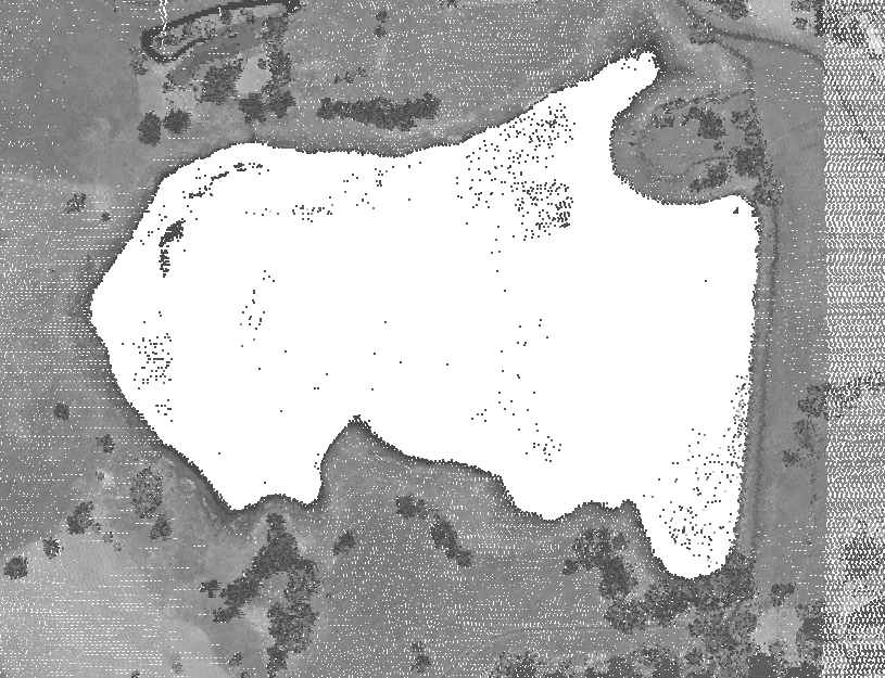
In Figure 1 is depicted a water body in the Boulder, Colorado area. This figure is rendered as points, colorized in gray by the LIDAR return intensity. These data have not been classified, yet it is obvious that this is a water body.
[1] This is an old database format called “dBase”
Figure 1: A water body shown rendered by intensity
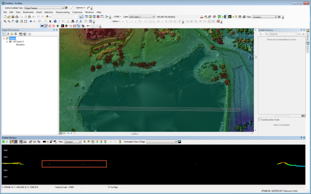
In Figure 2 is depicted the lake rendered as aevation color-coded triangulated irregular network (TIN), modulated by intensity. Notice several features of this water body. First, the water body is not “flat” as is evident by the shaded relief triangle facets that appear on the lake surface. Secondly, note the water points that are showing in the profile view. Due to vertical noise in the LIDAR and potentially wave action on the water body, these water points will not exhibit the same vertical values and hence will distort a TIN rendering of the surface. Finally note (from the profile graticule) that the elevation of this lake is about 1,872 meters above the vertical datum. Thus while we expect a water body to be flat, we do not (at least in general) expect the elevation to be at zero.
Figure 2: Lake rendered as a TIN with water points shown in the profile window
To flatten this water body, we must do several things:
- Construct a polygon that denotes the land-water boundary
- Provide a single elevation value to be used for designating the elevation of the water body
- Either remove all interior points from inclusion in the TIN or set their elevation values to the chosen water body elevation.
When following best practices in LIDAR data processing, the values of a LAS point’s X, Y and/or Z coordinates are never changed once past the rigorous geometric correction phase. Therefore we will eliminate the use of the interior water points rather than change their coordinate values (in fact, there is not a tool in LP360 that will allow you to change LAS point coordinates!).
The polygon used to demark the boundary will be either a 2D or 3D shape feature. As previously mentioned, it is possible to use a 2D feature for a flat surface since each vertex Z will be set to the same value and that value can be stored as an attribute.
The general class of tool used in LP360 for breakline creation and edit are the Conflation point cloud task (PCT) tools. These are accessed either directly as a PCT or (preferred) via the Feature Edit tools contained on the Feature Edit toolbar. Since this article is about breaklines rather than feature edit, I will concentrate directly on the PCT dialogs.
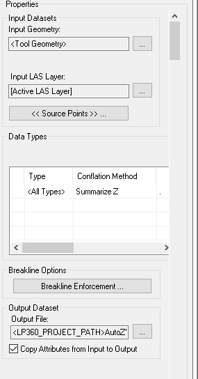
I will provide an example of extracting the Z value from the LIDAR as the method of resolving the elevation value to use for the lake surface. The Summarize Z method of conflation is used for this task (see Figure 3).
Figure 3: The Summarize Z dialog
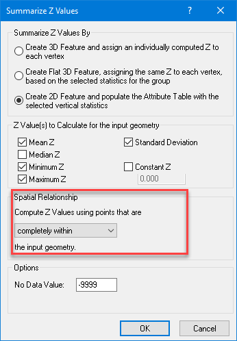
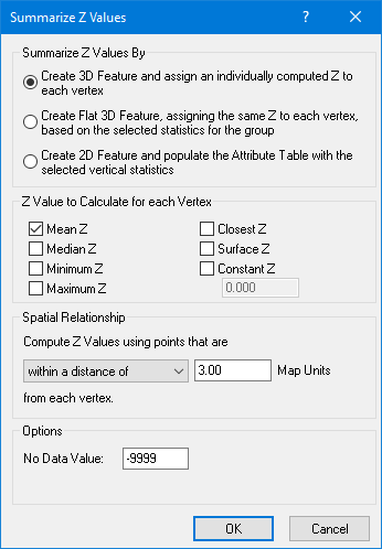
The settings dialog for the Summarize Z method is opened by clicking the ellipses to the right of the Summarize Z drop-down in Figure 3. This settings dialog is shown in Figure 4. Note that there are a number of methods of computing the Z value. If you know the value that you would like to use, you can simply check the Constant Z option and key in this value. You can also use statistics of points either within a range of the vertices or completely within the polygon that is to be drawn. I have set the method to use points completely within the polygon that I will draw. I chose this method since a visual inspection of the lake revealed that the interior points were relatively flat and should provide a reasonable estimate of the water surface level. Note that other methods are available that allow you to set a radius around each point and compute the statistics by including all points within the circle.
Note that I have elected to compute a single set of values and store these in the attribute table. If these attributes are not currently defined in the attribute table associated with the feature file defined as the output file in the task, they will be automated added (you no longer need to manually add attributes for feature digitizing).
I have chosen to compute Mean, Min, Max and Standard Deviation since, by examining the results, I can quickly detect if I have anomalies in the data that will affect the result. I have also added Standard Deviation since this value will provide an idea of how much variation in elevation exists in the water points.
Figure 4: Computing the Z value
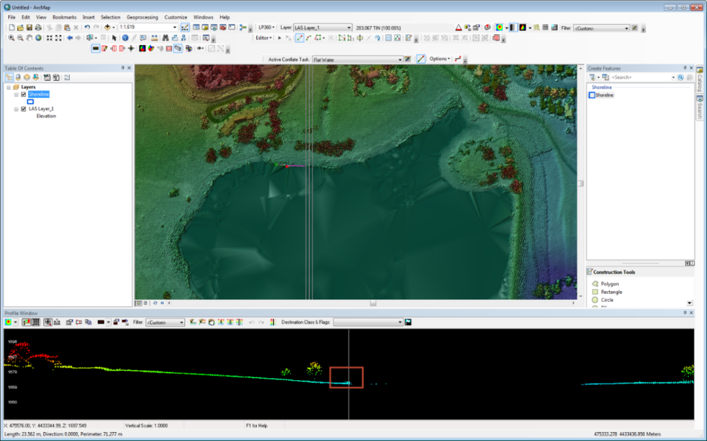
I now simply digitize the lake shore from the LIDAR TIN rendering. Note that LP360 combines the profile view with the Map View to allow you to easily see the true shore line. This is activated by pressing the “P” key while digitizing a breakline. A white vertical line is displayed in the profile view at the location where a point will be digitized in the Map View (see Figure 5).
Figure 5: Digitizing the shoreline (note the vertical white line in the profile view)
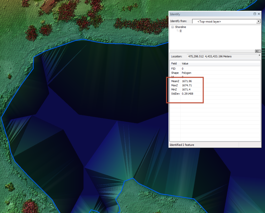
The resultant breakline and collected statistics are depicted in Figure 6 (I am using LP360’s Identify tool for a quick look at these data. I could use Feature Analyst for a more detailed inspection). Note that the system computed a mean Z value of 1,671.96 m with a standard deviation of 0.291 m. Due to the relatively small standard deviation, I am satisfied with this result and will apply the Mean Z as the elevation to use for the flattening operation.
The next step is to classify all of the interior points as Water points. Note that I could have done this concurrently with digitizing the breakline. However, I like to keep this as a separate “Classify by Feature” step in case I make a mistake in breakline digitizing and have to modify the feature.
The interior points are reclassified to water by using the “Classify by Feature” tool in LP360. I set the source class to All and the destination class to water (see the LP360 online help for details on this and the other operations in this article).
Figure 6: Breakline with collected statistics
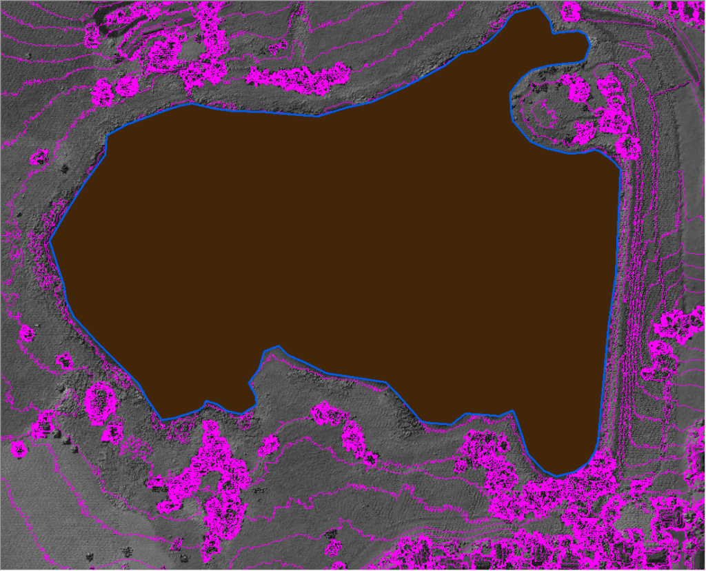
I am now ready to enforce my new breakline. In the breakline enforcement dialog, I set the “Buffer Class” to Water so that the water points are not included in the TIN surface. The result is depicted in Figure 7. Notice that the water surface is perfectly flat (in the TIN rendering) and that none of the contours cross the breakline.
To create a Digital Elevation Model (DEM) with the breaklines enforced, I simply use the Export Wizard in LP360, setting the breakline option the same as I have in this exercise. The result will be a gridded elevation model with flat water surfaces.
Figure 7: The enforced breakline
It is worth reviewing the Summarize Z methods in LP360. The dialog is depicted in Figure 8. The three options are:
- “Create 3D Feature …” – This option creates a 3D feature with a (potentially) different elevation value stored on each vertex. The options in the check box section act as “radio” buttons meaning only one can be selected. Depending on your selection, the Spatial Relationship section may be enabled. For example, if you chose Mean Z, the Spatial Relationship allows you to specify the radius of points to be used in the computation of the mean.
- “Create Flat 3D Feature…” – This option creates a 3D feature with the same elevation value assigned to each vertex. Once again, the options in the Z Value section become radio buttons. Here if you choose an option such as Mean Z, the mean Z for each vertex is computed based on the points contained within the radius set in the Spatial Relationship entry. These individual mean values are then averaged over all the digitized vertices and this final value is stored as the Z value for all vertices.
- “Create 2D Feature …” – This is the option we chose for the lake digitizing example. It functions similarly to the Flat 3D feature option except values are stored as attributes on the feature rather than on the vertices. Be careful in using this option if you intend to export your features for use in a 3rd party package other than ArcGIS. Not many CAD packages can extract geometry data from feature attributes.
Figure 8: Summarize Z dialog
See the final article in this series, Breaklines in LP360 – Part 5
