How to do power line classification and vegetation encroachment with LP360

1. Introduction

This article is a step by step tutorial on how to do power line classification and vegetation encroachment. The idea is to share a dataset example, with the PCT prepared for a user to test the tool and develop later his own workflow.

This article is the step by step tutorial of the article How to Classify Power Lines, it is recommended to watch the 10 minutes video before performing this workflow. There is more information is needed check this article How to identify powerline encroachment.

2. Pre-requisites

2.1. Licensing

This workflow requires LP360 Drone license plus Business Intelligence tools addon.
If you want to try the workflow, but you don’t have the correct license, please contact us to provide a demo license.

2.2. Data

I will use the following data as an example:

Download example dataset – TV535powerlines

But you can use any other data, the requisites are:
1. LiDAR data, where we can see powerlines. Towers + cables.
2. The point cloud should be processed. We recommend having a clean dataset before starting the workflow. Some tools you may want to use before are: Strip Adjustment, Smoothing, QA with control points, remove outliers…
3. It is recommended to have the ground classified, but it is not essential.
4. It is recommended to have a shapefile with the powerline path. It does not need to be very accurate, but it helps with the initial steps. It can be added as shapefile or KML.

2.3. Point Cloud Tasks

I will use the following PCTs, you can directly add the file with the settings I use for the example dataset:

Download PCTs – Powerline training

If you want to create your own PCT, we will use:

3. Workflow

The workflow is the following:

Configure in Feature edit, the Z to use the conflation tool.
Configure the feature analyst to zoom in the profile each vertex selected
Create a 3D polyline with the powerline path, make sure each vertex is the top of each tower. Optional, import a shape file with the path and edit it to create a 3D polyline that snaps in the top of each tower.
Classify manually each tower, they don’t need to be perfect, usually I classify until I see low vegetation or the ground.
QC the towers classification, If you are not happy with the result, use the PCT Tower to unclassified, and repeat step 4.
Perform Powerline extractor
QC the results using the feature analyst
If the results are not correct, use the PCT Wires to unclassified, and repeat step 6.
PCT Classify by feature 10 meters
PCT Classify by feature 7.5 meters
PCT Classify by feature 5 meters
PCT Cluster by distance.
PCT Tracing and squaring
Export final results

4. Step by step

1- Import data into LP360
2- Load the PCTs

4.1. Configure the conflagration for the Feature Edit

1- Go to Feature Edit ribbon
2- Feature Edit Options
3- Select in “Surface Auto-Z Settings” –> Edit feature conflation task: 09_Snap_to_Tower –> Create Feature conflation task: 09_Snap_to_Tower
4- Press OK

If you need to configure you own PCT:

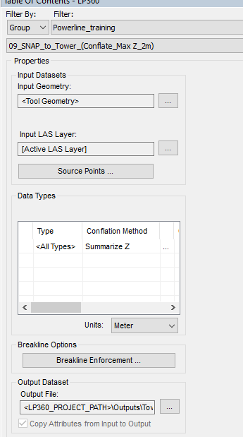
09_Snap_to_Tower

Conflation PCT
Input Geometry–> Tool Geometry
Input LAS –> Active LAS layer
Source points –> All
Data types –>Summarize Z
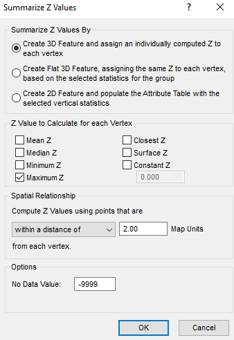
Summarize Z Values:
Checked –> Create ·D Feature and assign an individually computed Z to each vertex
Checked–> Maximum Z
Compute Z Values using points that are –> within a distance of–> 2 map units (2 meters for the example, in case of feet select 6)
No Data Value–> -9999
Output file–> Project path\Outputs\locations.shp

4.2. Create the powerline corridor

Option 1: Add the corridor from a KML or shape file–> Edit the file to make it 3D polyline –> Conflate every vertex to the top of a tower

Option 2: Create your own shapefile

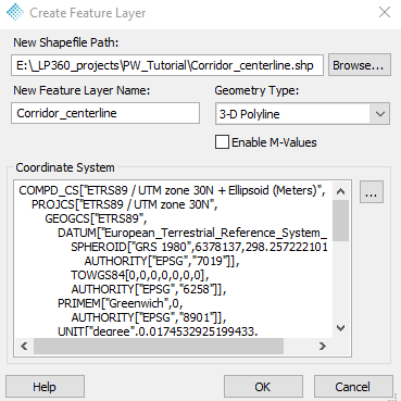
1- Go to feature edit –> Create Feature layer –> 3D Polyline

2- Change the point cloud view to by elevation
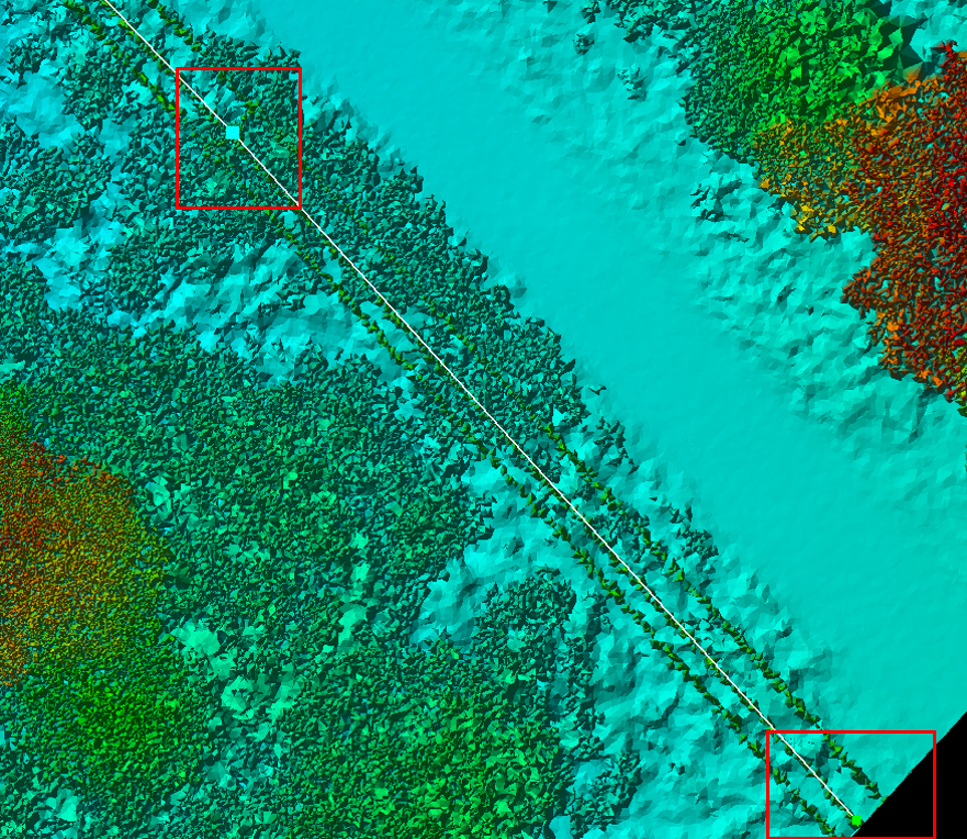
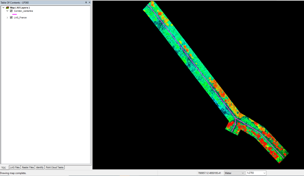
3- Press Create Feature –> Click in the beginning of the powerline–> Click again in the top of the first tower. This will create a line, continue clicking in the top of each tower to create the centerline. If there is more than one direction. After you finish with the main line, create a another line for the second direction.
Note, all the lines needs to be contain the same layer. After you finish, press right click “finish edit”

4- Save edits

At this point we have a shapefile with the powerline corridor. It is a 3D polyline with each vertex in the top of each tower.

4.3. Configure the feature analyst

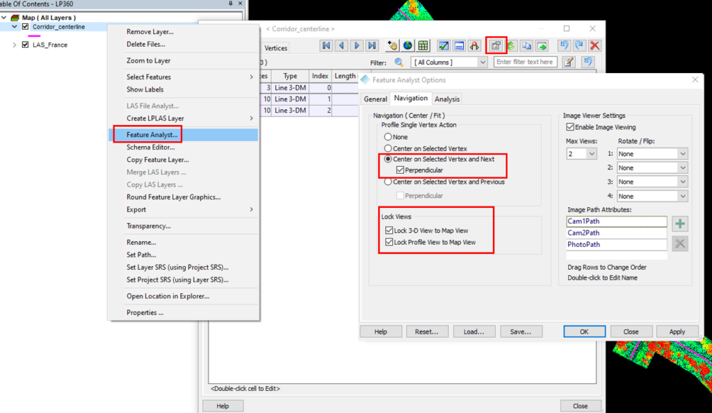
Right click in our “corridor” shapefile –> Feature Analyst –> Feature Analyst Options –>
–> Center on Selected Vertex and Next –> Lock 3D View to Map View –> Lock Profile View to Map View –> OK

4.4. Classify the transmission towers

1- Create a profile perpendicular to the first tower. Make sure to cover all the tower with the depth.
2- In the profile, view by classification –> Classify by polygon –> Destination “15 Transmission Tower”
3- Create a polygon around the tower, and press two times space to classify.

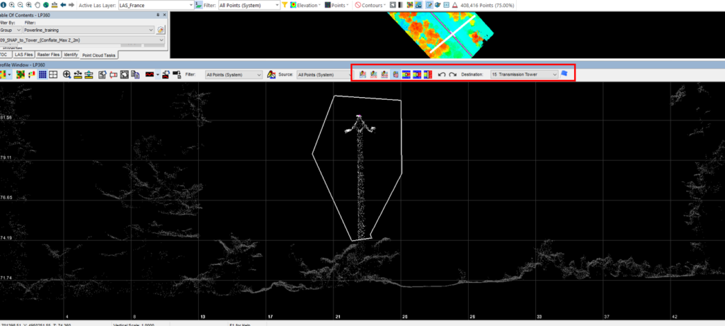
4- Keep the profile windows open. Open the “Corridor_centerline” Feature analyst –>”Select a feature”–> Go to “Vertices” –> Select the second “Vertice”
5- The profile view will navigate till the first tower, continue with the tower classification

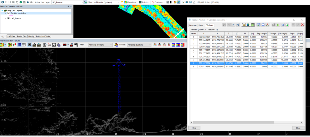
6- After you finish with the tower classification, we pass to the next step. Wire classification.

4.5. Powerlines classification

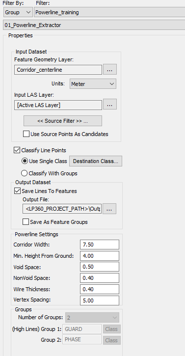
1- Open the PCT Powerline_extractor.
Use the following settings:
– Feature Geometry–> Corridor_centerline.shp file (the layer with the 3D polyline created in step 4.2.)
– Classify Line Points –> Use Single Class –> Layer 14 wire
– Output –> Check Save Lines to Features –> Add an output folder
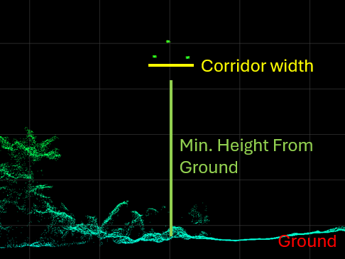
– Powerline profile settings

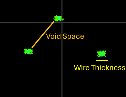
Powerline settings:

Note: Wire thickness is the thickness of the cable in the point cloud. The NonVoid Space will be always the same value as Wire Thickness. Vertex Spacing is the distance between vertex in the 3D modelled wire.

2- Run the PCT Poweline Extractor –> “By Active Layer”
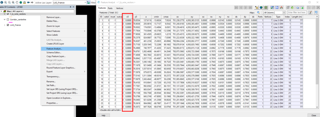
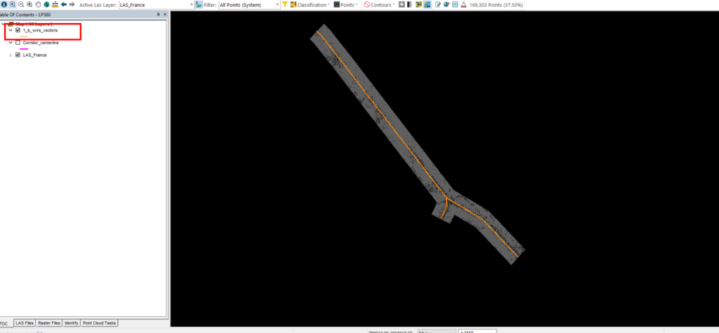
3- Now we will have the wires extracted and the wires points classified. The default PCT create a wire called, 1_b_wire_vector layer.
4- Perform QC of the wires –> Go to the Wire_vector layer –> Feature analyst –> Check the x0 column.
Organize the values from Max to min, and later from min to Max.
– If the x0 values is next to 0 the catenary is good.
– If the x0 values is different than 0, for example 85 or -100. Then the catenary is bad.

5- Go to all the catenaries with large x0 values, QC and delete them.
6- After that go to feature edit –> Press “Save edits”
7- If you find the classification or the wire was not properly model. Use the PCT Wire to unclassified, and repeat step 2.
After this point we should have all our cables classified and modelled in a shape file

4.6. Vegetation encroachment

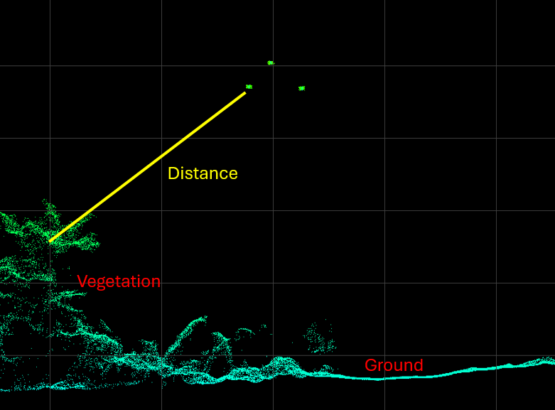
After we have our cables model in 3D, we can perform the vegetation encroachment. To do this step we will ask the software to calculate all the points that are within a radius of the wires. If we use more than one radius, we will perform this step from the biggest radius to the smaller.

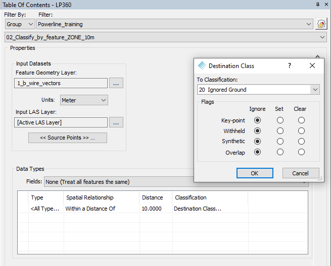
We will use the PCT 02_CLassify_by_feature_ZONE_10m, 03_CLassify_by_feature_ZONE_7.5m and 03_CLassify_by_feature_ZONE_5m.
However you can create you own PCT for different radius.

PCT Classify by feature biggest radius – 10m
PCT name–> Classify by feature
Feature Geometry Layer–>”1_b_wire_vector” (the wires extracted from the powerline extractor)
Source points–> Unclassified
Type–> All types
Spatial Relationship–> Within a Distance Of
Distance–> 10 (change this value depending the radius)
Destination Class –>20 (use a different class for each radius)

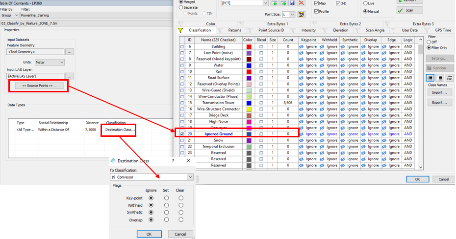
Explanation of the classify by feature settings

PCT Classify by feature next radius – 7.5m
PCT name–> Classify by feature
Feature Geometry Layer–>”1_b_wire_vector” (the wires extracted from the powerline extractor)
Source points –> 20 Ignored Ground (in the seconds radius all the points will already be included in the previous radius).
Type –> All types
Spatial Relationship –> Within a Distance Of
Distance –> 7.5
Destination Class –>21

1- Perform PCT 02_CLassify_by_feature_ZONE_10m –> Select As a feature Geometry “1_b_wire_vector” (the wires extracted from the powerline extractor)
2- Perform PCT 03_CLassify_by_feature_ZONE_7.5m –> Select As a feature Geometry “1_b_wire_vector”
3- Perform PCT 04_CLassify_by_feature_ZONE_5m –> Select As a feature Geometry “1_b_wire_vector”

After this step we will have classified all the points with vegetation closer than our Zones. In the example: 10, 7.5 and 5 meters.

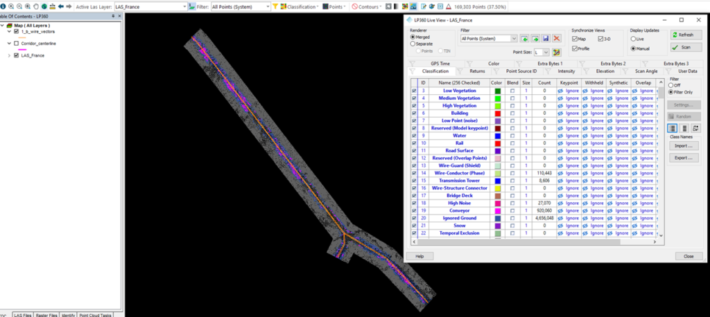
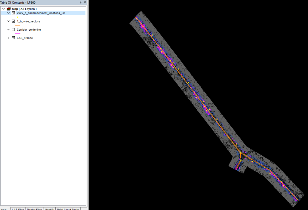
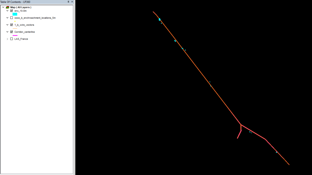
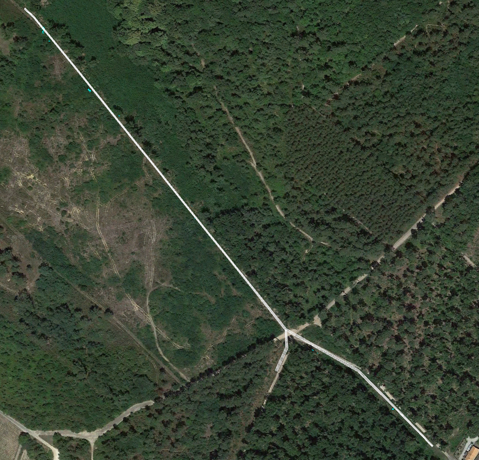
In the latest screenshot, we can see:
– The cables vectorized in a shape file, orange lines
– The vegetation encroachment, in the map we see multiple colours around the powerlines.
– Live View, if we scan the LAS. We can see points in the layers:
14 Wire
15 Transmission towers
18 Encroachment Zone 5 meters
19 Encroachment Zone 7.5 meters
20 Encroachment Zone 10 meters

Now we will move the to export part of the workflow.

4.7. Export points

The first thing we will export is a shape file with the locations where the vegetation is closer to 5 meters to the cables.

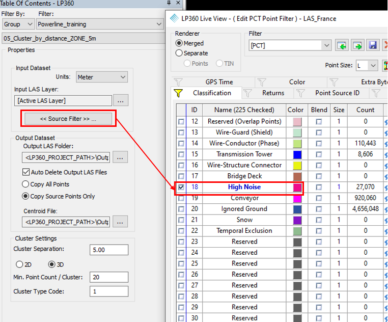
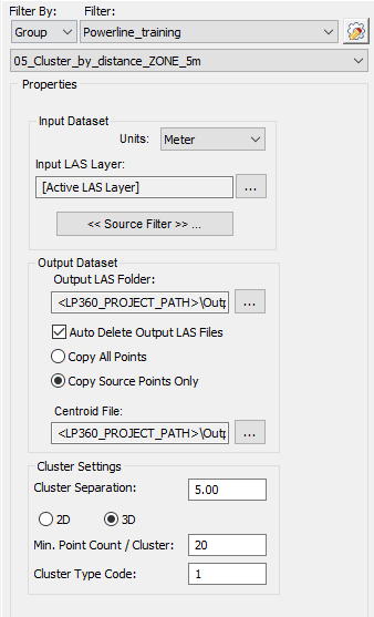
We will use the PCT 05_Cluster_by_distance_ZONE_5m

PCT Cluster by distance
PCT name–> Cluster by distance
Source Points –> layer 18 (the layer with our 5 meters radius information)
Output LAS Folder –> Add a folder (this output will be deleted automatically)
Check Auto Delete Output LAS Files
Centroid File –> Add a location (this is the shape file with the location)
Cluster Separation –>5
3D
Min Points Count –> 20
Cluster Type Code –> 1

1- Perform PCT 05_Cluster_by_distance_Zone_5m

It will create a layer with points, all this points are areas where the vegetation is closer to 5 meters.
After this, we can select the layer –> Right click –>Export –> Export as KML

4.8. Export polygons

Another way to export the results is to create polygons in the areas where the vegetation is closer than 5 meters.

We will use the PCT 06_Point_Group_Tracing_Zone_5m

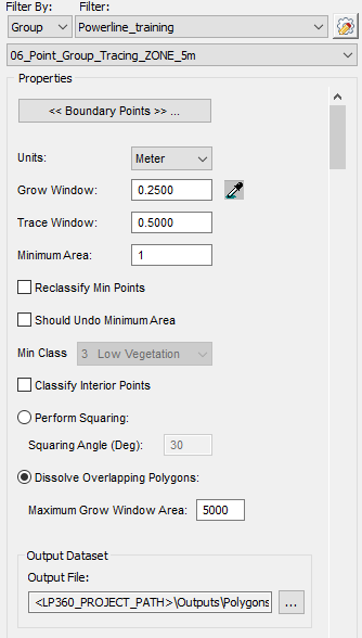
PCT Point Group Tracing and Squaring
PCT name–> PCT Point Group Tracing and Squaring
Boundary Points –> layer 18 (the layer with our 5 meters radius information)
Grown Window –>0.25
Trace Window –> 0.5
Minimum Area –> 1
Dissolve Overlapping Polygons:
Maximum Grow Window Area –> 5000
Output File –> Add a folder (this is the shape file with the location with the polygons)

1- Perform PCT 06_Point_Group_Tracing_Zone_5m

t will create a layer with polygons, all this polygons are areas where the vegetation is closer to 5 meters.
After this, we can select the layer –> Right click –>Export –> Export as KML