This article is a continuation of the discussion of breaklines in LP360 (the standalone version). In last month’s installment, we discussed the overall concept of data modeling, especially the Triangulated Irregular Network (TIN). In this installment, I will discuss the general concept of adding constraints in the form of breaklines to these models. In future installments, I will examine the various methods of breakline collection and enforcement that we have enabled in LP360.
1 An Overview of Breaklines
A breakline is a vector-based feature (a point, polyline or polygon) added to a 3D model. A more generic (and correct) term would be a supplemental model constraint since, in addition to 3D lines, LP360 supports points and polygons. However, breakline is the accepted terminology in the mapping industry and the one I will use in this paper.
Breaklines are two or three-dimensional features (generally polylines or polygons) introduced into the TIN to constrain the generation of surface models. These introduced breaklines may be developed such that they do not modify the original surface geometry (“soft” breaklines) or to add “deflecting” elevation points to the surface (“hard” breaklines). Breaklines can be stored as ancillary feature data that are dynamically added to the model when needed (during surface generation or derived product creation). Alternatively, breaklines can be “burned” in to the surface model as strategically placed points (sometimes referred to as “Steiner” points) that are flagged as “model key points.” A model key point is a point that is flagged to always be retained in a model during thinning processes. Dynamic modeling, while much more difficult to implement in software, is far more flexible in interactive modeling situations (e.g. change, observe, change, observe, …). LP360 implements this advanced approach to dynamic breakline modeling.
2 Soft Breaklines
In this and the next section I discuss Hard and Soft breaklines. I actually do not like this terminology because it is not well defined. In general, breaklines of any type can modify the surface model and thus there seems little point in making a distinction. Historically this distinction has been made so it warrants a bit of discussion.
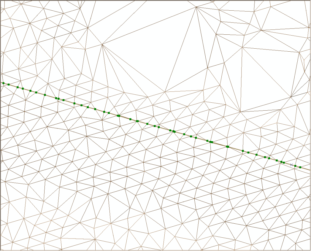
Breaklines introduced into a surface such that none of the existing TIN elevations are modified are termed “soft.” These breaklines are used to preserve original elevations in a model or to indicate a feature in the TIN such as the edge of a road. Figure 1 depicts a soft breakline being introduced to demark the edge of a road. Note that a vertex has been inserted (green nodes) at each intersection between the line segment and the TIN. Each of these nodes will take on a Z value identical to the elevation of the intersected triangle edge. Points that are digitized in the process of creating the line that do not fall on a vertex (which is most of them) are “snapped” to the surface of the facets of the TIN. This operation is termed a “pure drape.” This is quite a visual term as you can see how the line has been “draped” over the TIN. Note that since we have not yet “enforced” this breakline, the triangles intersected by the line segment have not been modified.
Figure 1: Introduction of a soft breakline (unenforced)
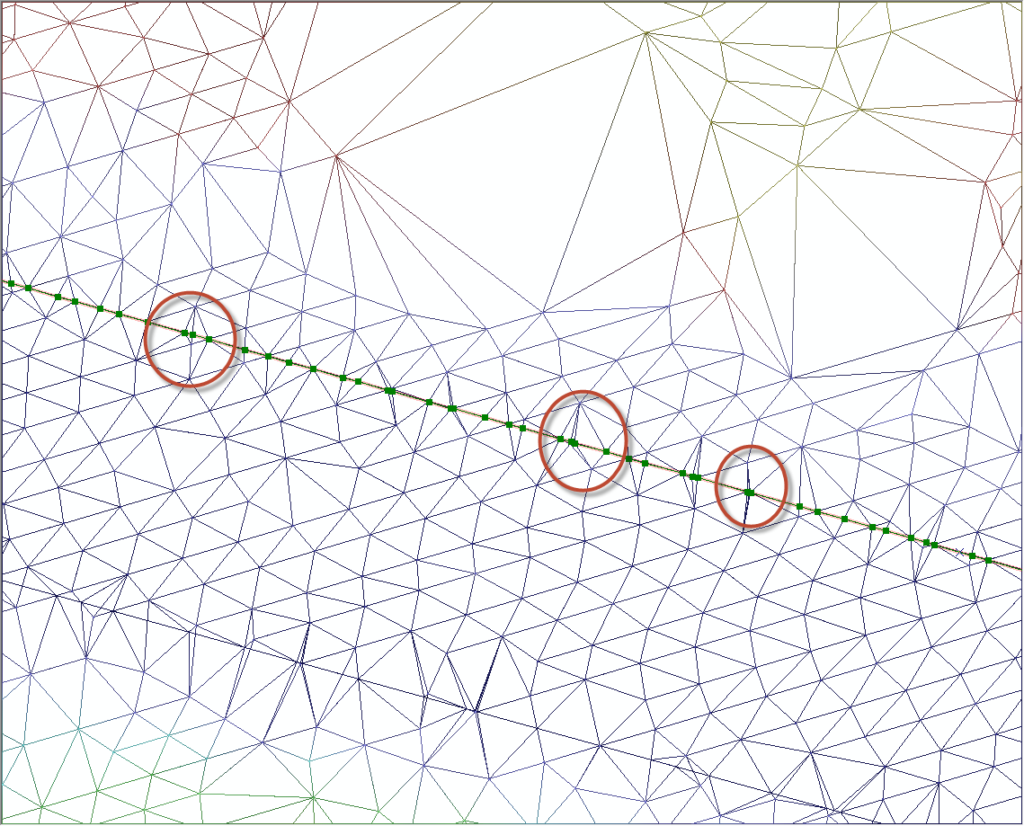
Figure 2 shows the reconstructed TIN after introduction of the breakline. Note that the elevation of each introduced node is interpolated from the edges of the original TIN of Figure 1 at the point where the line crosses the TIN edge. That is, a new node (also referred to as a vertex) is created at each point where one of the introduced lines crosses an edge of the original TIN. This new model will very closely resemble the original model since we have not introduced any new elevation points. However, there are subtle differences because enforcing the breakline introduces a new triangle vertex at each point where the line crossed an edge of the original TIN. This breakline enforcement forces the new TIN to violate the previously mentioned Delaunay criteria because it forces triangle edges to be inserted along the breakline. These areas of “redundant” triangle construction are denoted by the red circled areas in Figure 2.
Figure 2: Depiction of the TIN after enforcing the breakline
Note that even though these “soft” or draped breaklines do not introduce any changes in terms of elevation points, the change in the triangulation (as depicted in Figure 2) can cause very subtle changes in the elevation models that will be derived from the TIN. Figure 3 shows the small change in contour position that results when enforcing the breakline. In most cases, the changes in contours introduced with soft breaklines will be very small (the contour interval in Figure 3 is only 0.2 feet).
 |
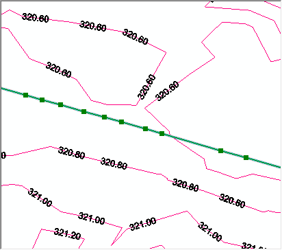 |
Figure 3: Unenforced (left), Enforced (right)
Soft breaklines generally serve several functions. Firstly, they preserve the topography as subsequent operations are performed. For example, withholding some of the ground points after introducing the soft breaklines of our example (most typically in a data thinning operation) can dramatically change the morphology in the neighborhood of the breakline but it will not change right at the line. A second reason for introducing soft breaklines is to force a correct morphology at a known break edge. A good example is the crown of a road. Since LIDAR points fall at pseudo-random locations on a surface, there will not be a nice line of points directly on the road crown. Draping a breakline directly on top of the crown will ensure that this critically important feature is preserved. Another consideration is the use of “soft” breaklines for feature coding operations. Sometimes the facets of triangles are labeled with a feature class such as “Ground” or “Road.” Introducing a soft breakline allows one to split features such as the Ground into two features (Ground, Road).
3 Hard Breaklines
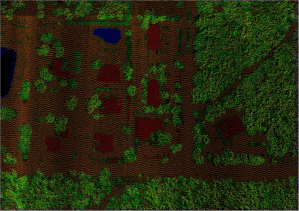
As we have discussed in the previous sections, breaklines are two or three-dimensional graphic data (points, lines, polygons) that we introduce into an elevation model to alter the topology. When working with Geographical Information System (GIS) models, we nearly always model complex, irregular elevation data as a Triangulated Irregular Network (TIN). The source of the elevation points need not be from a LIDAR sensor. Surveyed mass points, scanned contour lines, correlated stereo models and myriad other sources produce irregular elevation data that can be modeled as a TIN and tools (such as LP360) that can manipulate random points are generally adept at processing these various data sources. Figure 4 is a point rendering of a typical airborne LIDAR scene that has been processed via automatic classification in LP360 (but not interactively edited). Note that due to the high point density in this particular data set, features are recognizable even though the point cloud provides a fairly crude rendering.
Figure 4: Points from a LIDAR Scene (data courtesy of Southwest Florida Water Management District)
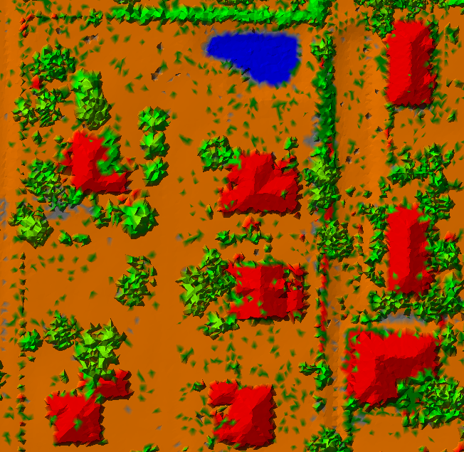
Recall from our previous discussions that a TIN is a convenient way to model point data because we can construct a solid surface (by filling in the triangle faces or facets) and include every point. No other geometry provides us this important capability. Note that we can even model “wrap-around’ surfaces such as the faces of tunnels with a TIN so long as the TIN is a true 3D construct. Figure 5 is the same scene as Figure 4 but now rendered as a TIN. As you can see, the TIN generally provides a much richer viewing context.
Figure 5: A TIN visualization
Breaklines allow us to modify the rendering of a TIN (as well as the extraction of ‘derived’ products from the elevation model). We discussed the idea of a soft (sometimes referred to as a 2-dimensional, 2-D) breakline in the first part of this paper. Recall that a soft breakline, while potentially altering the node placements in a TIN, does not deflect the TIN from the surface defined by the point cloud alone. These soft breaklines can be collected using a wide variety of methods from field surveys to heads-up digitizing from a digital orthophoto.
A “hard” breakline modifies the elevation of a TIN by introducing auxiliary “Z” (elevation) points in a constrained manner where these added points are above and below the original TIN surface. Before we dive in to the details of what exactly is meant by this last sentence, let’s consider how we obtain these 3D vectors. I will refer to graphical objects that are represented by nodes and lines as vectors even though this is not technically the definition of a vector! This is a hold-over from differentiating computer displays based on raster or line drawing techniques.
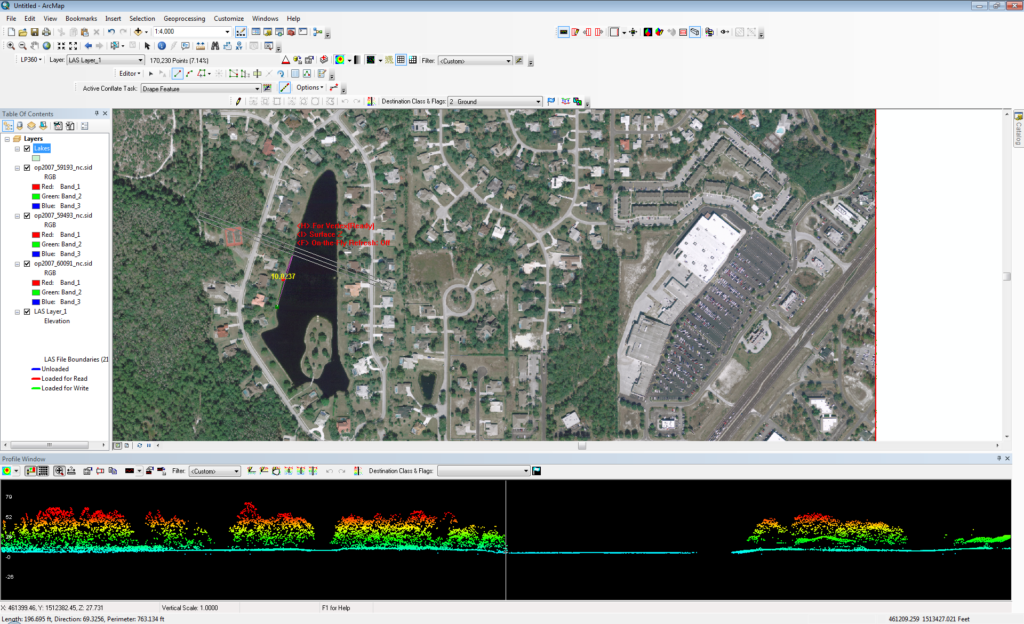
In order to enforce 3D constraints in an elevation model, we need 3D vectors. One of the huge advantages of LIDAR data is its very high vertical accuracy. 10 cm or better vertical network (sometimes called “absolute”) accuracy is now commonplace in wide area aerial mapping. Therefore, we can often use the LIDAR data themselves to enforce elevation models derived from the LIDAR data (this circular idea is the subject for another paper!). A very common scenario is to digitize the planimetric (X, Y) portions of the vectors from a digital orthophoto and attribute the Z value from LIDAR. This process of creating a composite feature from multiple sources is termed “conflation.” LP360 (both the ArcMap and Windows versions) contains a rich set of tools for conflating Z values onto 2 dimensional vectors and for densifying existing 3D geometries. For example, Figure 6 illustrates dynamic conflation using ortho photos for the planimetric capture and LIDAR for the Z component. Note that I am digitizing a lake feature in the Map View of LP360 while simultaneously viewing the vertical dimension in the LP360 Profile window. Not only does this allow me to much more accurately trace the shore line (by keeping the vertical white line in the profile view aligned with the shore) but the Z (vertical) component of my 3D shore line vector is being automatically populated from the LIDAR data via the Conflation process. This process is a very practical form of data fusion.
Figure 6: Dynamic Conflation using a high resolution ortho and high-resolution LIDAR
See the next article in this series, Breaklines in LP360 – Part 3
