Introduction to Part 3:
In the last part of this series, we discussed in some detail how a Triangulated Irregular Network (TIN) can be constrained by features external to the point cloud model such as lines, points and polygons. In this month’s edition, we will look at contours and how LP360 can extract elevation information from point cloud data for assigning to the Z component of feature vertices.
Contours:
Before we delve in to exactly how breaklines are collected, it is useful to review contours and how they are generated from a TIN. A contour is a mathematical concept. It is generally a curve along which a function of two variables has a constant value (also called an “isoline”). In terrain modeling, we can express the elevation, z, at any point (x, y) as a function of that planimetric location; z = f(x, y). Thus an elevation contour is a line in x, y along which the value of z remains a constant. We can write this mathematically as Ci = f(x, y) where the index on C indicates a specific contour.
If you walk along a contour line, you will never move up or down. In Figure 1 is illustrated a contour rendering (using dynamic contouring in LP360) of an open pit mine. The 1,650’ contour is indicated by the red arrow. If you were to walk around this mine, staying on the contour (not recommended!), you would move in the x, y plane but not up or down. If you pour water on a contour, it will move in a direction perpendicular (“normal”) to the contour line.
Figure 1: Mine Contours with 1,650’ contour line indicated (point data courtesy Trimble)
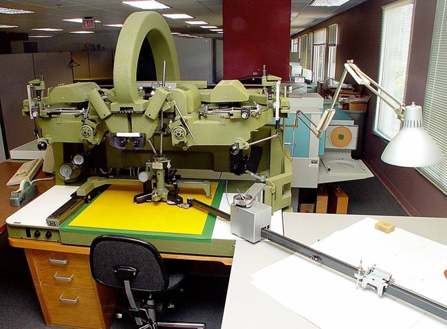
Back in the old days of cartography (way before my days!), contour data were directly collected from the field using survey techniques or from aerial photos (film, not digital) using stereo plotters. Stereo plotters were huge optical-mechanical devices that allowed the user to directly trace contours while looking at the overlapping stereo photos through a binocular optic. An example of one of these beasts is shown in Figure 2. The United States Geological Survey (USGS) had collected elevation data for the entire United States as contour lines. These were published in the USGS topographic map series (USGS Quad Sheets). These maps were printed from map “separates”; sheets of photographic film the size of the quad sheet with each layer containing a “theme” that would be printed in a single color. The contour layer was one of these separates.
Figure 2: Stereo plotter set up for tracing
In the 1980’s, the USGS embarked on a massive program to convert the map separates (these pieces of film) to digital format. This conversion was not simply to generate unintelligent raster graphics but to actually convert this essentially “picture” data into intelligent digital mapping data. One portion of this program was to scan the contour separates and, via mathematical algorithms, convert the scanned contour lines into Digital Elevation Models (DEM). Some of this original conversion software is still available in the open source Geographic Resources Analysis Support System (GRASS) software. Much of this converted data still comprises the USGS DEM database! Thus when you obtain elevation data from the USGS national holdings, you may well be using scan converted data from the original quad sheets!
I hope you notice the irony in the overall situation. In the beginning, we collected contours by direct survey or by manual tracing from stereo imagery. We then developed scanning and conversion technology to convert this line work to digital elevation “posts.” Today, we directly collect elevation posting using LIDAR or dense image matching. We then use contouring algorithms to generate line work – the circle is complete!
So if we did all of this work back in the 1980s and 1990s to convert contour line work to digital elevation posts, are contours of any remaining practical value? A few years ago, I thought that the answer was a marginal yes. This was when I dealt mostly with the production side of elevation data processing. However, since moving into the exploitation side of elevation modeling by our acquisition of QCoherent Software (way back in 2009) and my subsequent involvement in developing new algorithms in this arena, I have gained a renewed appreciation for the contour. While 3D visualization is definitely the way to visualize 3D data, the contour provides an extremely useful visualization tool when superimposed on a 2D model. I think you will agree that it adds a lot to the visual comprehension experience, even when viewing a 3D model. We discussed this in the March 2013 issue of LP360 News. I have repeated an image from that issue as Figure 3 where you can clearly see, by the deflected contours, the drainage area in the lower left area of the image.
Figure 3: Adding vertical visualization to a a two-dimensional image
So what does all of this have to do with breaklines, the original theme of this current series? Well, contours are a very good tool for analyzing the behavior of constrained elevation models. For example, if we have a non-flowing water body (for example a pond) surrounded by land, we expect the surface of the water body to be flat. If it were not flat, the water would be flowing, violating the “hydro” constraint we placed on our model. Visualizing the contour lines surrounding the water body provides a very quick and intuitive means of validating the elevation surface. Figure 4 depicts a TIN rendering of a LIDAR project area with an enforced water body breakline. Notice how the contours follow the shoreline and do not cross the water body.
Figure 4: Enforced water body breakline
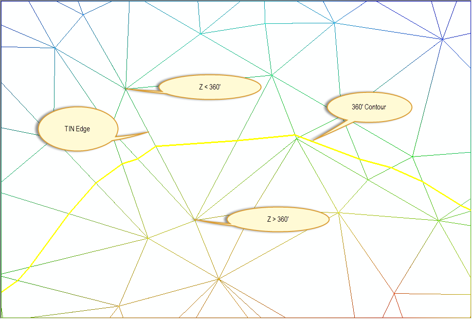
It is instructive to know how the contours are constructed. A common algorithm (used in LP360) is to find where a desired contour crosses an edge of the TIN representation of the point data. This is illustrated in Figure 5 for the contour at 360 feet.
Figure 5: Drawing a Contour
Conceptually (it is not actually done in this manner for performance reasons) a contour is traced throughout the TIN mesh. If one node of an edge is above the desired contour elevation and the other node of the edge is below the contour elevation, the contour must cross that edge. For example, when tracing the 360’ contour, if we encounter a node at an elevation of 358’ and an edge connected node at 362’, we know the contour must cross this edge. Of course, it is not sufficient to trace this single contour since the project area can contain many contours at the 360’ level. This means that every triangle must be inspected for an edge crossing.
Elevation models can be constrained by inserting edges that model the desired (or, more accurately, the true) behavior of the data. For example, to model a flat water body, we need a set of connected edges surrounding the water body with each node at the water body elevation. This modeling of elevation surfaces using breaklines is the subject of the next section.
Extracting Z from Point Cloud Data:
By now a natural question should occur; how exactly are the Z values being computed from the point cloud data? There are quite a few algorithms for doing this. LP360 supports a robust set for dealing with common situations. As time goes forward we will be adding more to the library.
- Pure Drape – This is a common technique that is used when you want a 3D line to exactly follow the surface of a TIN. The line work is “draped” over the TIN and vertices are directly computed from the line, TIN intersection. LP360 supports a variety of population schemes including keeping the original vector vertex spacing, inserting new vertices at a user-defined interval or inserting vertices where the vector crosses TIN edges. A pure drape creates a soft breakline so long as the same points are included in the model during the drape as will be included when enforcing the breakline.
- Downstream Constraint – This is a drape method that ensures that the vector monotonically decreases (or increases, depending on digitizing direction) from vertex to vertex. Thus it is enforcing a “correct” water flow. Obviously this requires excursions above and below the TIN surface. LP360 allows you to control the maximum excursions so as not to exceed a surface error tolerance. Figure 6 provides an example of a downstream constraint. The ground points are depicted in yellow. The constrained feature created by LP360 is blue. Notice in the area circled in red that the constrained feature had to be moved below the point cloud surface to enforce the monotonically decreasing rule. LP360 has triggers that will alert you if the deviation from the point cloud surface exceeds a specified error tolerance.
Figure 6: Downstream Constraint (ground is yellow, constrained vector is blue)
- Constant Z – This mode computes a value for elevation and then applies this value to all the vertices of the feature. Since a constant is being used, this value can also be stored in the attribute table associated with the feature. A constant Z algorithm is typically used for water body “flattening.”
Summarize Z – These methods use statistical or surface modeling techniques to compute a Z value. The method selected depends on the type of breakline you are creating as well as the quality of the point cloud data being used. We support a wide variety of options that comprise various combination of:
- Highest, Lowest Z – This method looks in a radial direction a user-specified distance from the vertex and locates the highest or lowest elevation point. An example might be digitizing a ridge line in an area of grass. Since many LIDAR pulses will reflect from grass, a “lowest” Z algorithm might be appropriate.
- Average Z – This method is similar to the previous method except that all of the points within the user-specified radius are averaged and this average Z is used. This can be useful for point cloud data over hard surfaces where your desire is to either average out noise or average out local slope.
- Closest Z – This selects the point closest to the vertex.
- Surface Z – This method simply interpolates the Z from the TIN facet. It is similar to a drape but it does not insert extra vertices at TIN edge
In addition to the above methods of computing Z, we also support a retaining wall method. This special method constructs, from a single input line, a set of two parallel lines a user-specified distance apart. These lines then have Z attributed based on both a high and low Z algorithm. The result is a line that represents the base of the wall and a second line that represents the top of the wall.
As you can imagine, there are all sorts of options with each of the above methods that allow you to tailor to many different situations. Some of the more common breakline collection scenarios for which LP360 is used include:
- Water Body Flattening
- Hydro-correct streams (down-stream constraints)
- Double line drain (River flattening – a scheme whereby the river flows downstream but opposite banks are at the same elevation)
With release 2017.1 of LP360 (the standalone version, not the ArcGIS extension) we added a new toolbar called “Feature Edit.” This collection of tools provides a very fast and efficient set of techniques for both creating and editing 3D features whose vertices are based on point cloud data. We have published several articles that detail the use of Feature Editor so make sure you check those out. These new tools are definitely worth the time you will invest in learning their use.
In next month’s edition, we will go in to detail regarding using Feature Edit tools to construct breaklines.


