1. Introduction
This article is meant to guide new LiDAR UAV users on how to process with LP360. This workflow is recommended for any LiDAR UAV user, sensors manufactured for example by Inertial Labs, Greenvalley, Tersus, Yellowscan, Fenix LiDAR or any other LiDAR UAV manufacturer. This workflow is different than TrueView, Microdrones, DJI L1/L2 or Wingtra. We’ve included a step-by-step guide to assist you with your processing.
2. Import
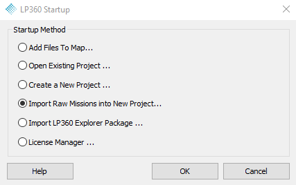
1- Open LP360
2- Select “Import Raw Missions into New Project…”
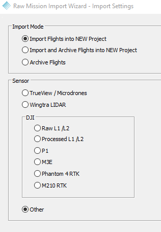
3- Select “Other”
4- Select the “LAS” and “Trajectory file” from your LiDAR processing software, we are looking for the trajectory file and LAS.
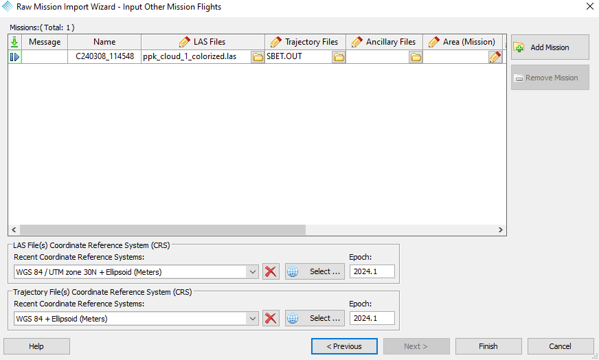
Where to find the files?
– LAS –> Point Clouds in LAS format
– Trajectory file –> Trajectory processing, INS, POS or Navigation folder.
The Trajectory file format can be in .out (sbet), .Post or .txt (ASCII).
Remember the correct CRS for each file selected in LiDAR processing software. The most common are:
– LAS in WGS84 UTM zone XX ellipsoidal heigh in meters, with epoch in flight date or 2010
– Trajectory in WGS84 ellipsoidal heigh in meters, with epoch in flight date or 2010
Note: If the LAS file does not contain the exact date information, a window will appear asking for the flight date.
5- Select the project output folder
6- Select the project CRS. This is the desired project CRS, it does not need to match with the input data CRS.
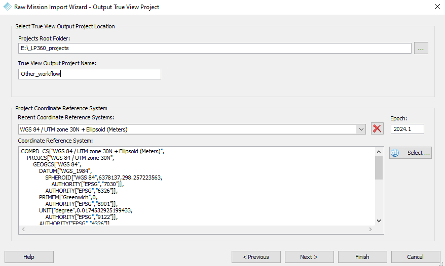
7- Press Finish
3. Point cloud generation
3.1. Flight lines generation
1- Go to Sensor ribbon
2- Auto Create Flight lines –> Compute Flight lines
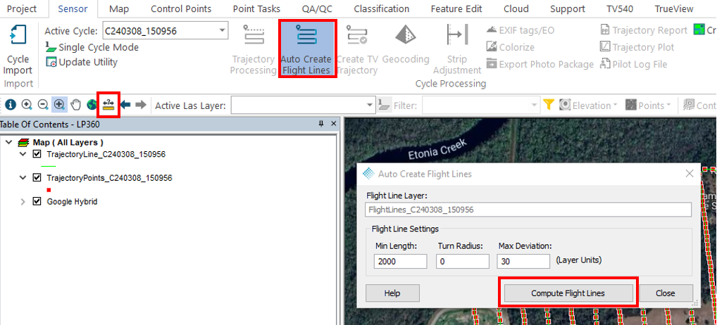
Tip:
– Use the “Measure” tool to learn approximately the flight line length.
– Make the “Min. Length” smaller than the smallest flight line.
– Make “Max. Deviation” bigger if terrain following is used. The example is in feet.
Note: screenshot example in US feet not in meters.
4- Select the undesired flight lines and delete them.
5- Feature Edit –>Select –> Click on the flight lines –> Press “delete” in your keyboard
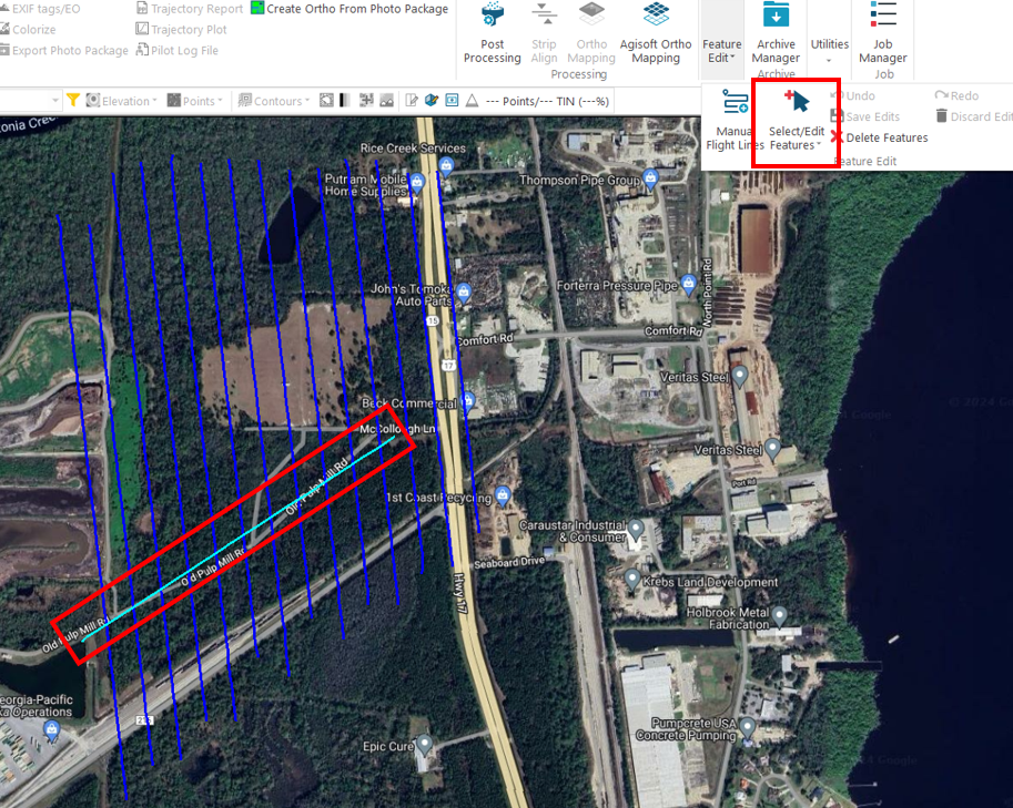
Tip: It is possible to create manual flight lines.
3.2. Post Processing point cloud
1- Go to Sensor ribbon –> Post Processing tool
2- Select the Clip Angle
Tip: clip angles is 50% of the FOV, if we select 40 deg clip angle means 80 deg FOV.
3- Select the Clip Range
Tip: If you want to generate all the points with no filter, uncheck “Clip Angle” and “Clip Range”.
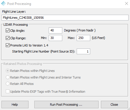
4- Run Post Processing …
Post processing will generate a new point cloud with the following attributes:
– Reprojected point cloud in the desired CRS
– LAS updated to the latest version (LAS 1.4)
– LAS divided by flight lines
– LAS with filters applied, clip angle and range
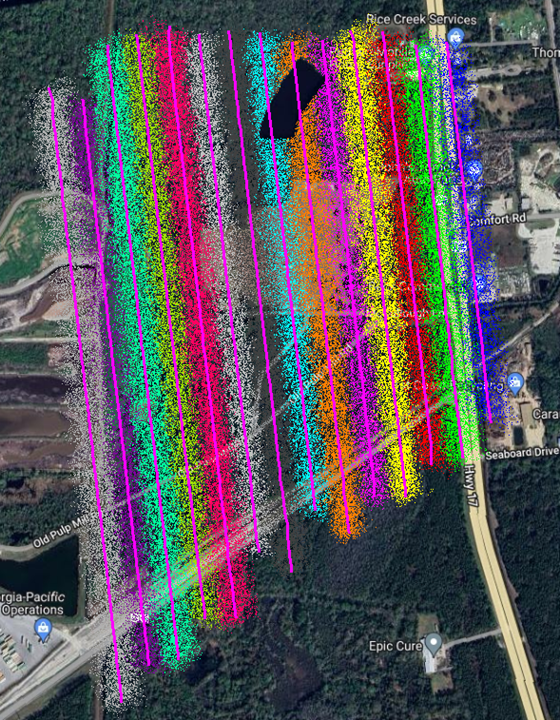
4. Strip Align
The next step will be to verify the alignment of the flight lines and correct it. For that we should perform cross sections in the overlap areas between flight lines. It is recommended to perform this sections in flat areas, buildings are especially useful for it.
We can also use tools like “Surface Precision” to verify the alignment across the flight or between multiple flights. After we have verify the alignment, we proceed to correct it.
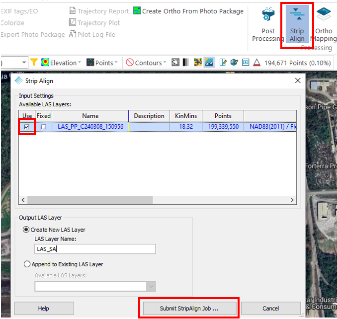
Strip Align tool requires the license addon “Strip Align“
1- Go to Sensor ribbon –> Strip Align
2- Select the LAS to align.
Tip: You can select multiple flights. If you do it, the tool will correct any misalignment between flights. However, if one flight has significant error (or bias), it will introduce error into the new Strip Align layer.
3- Press “Submit Strip Align job”
4- Go to “Job manager” –> Check the processing status
5- Once Strip Align finish the status will change to “Post process” –> Select the job–> Click “Post process”
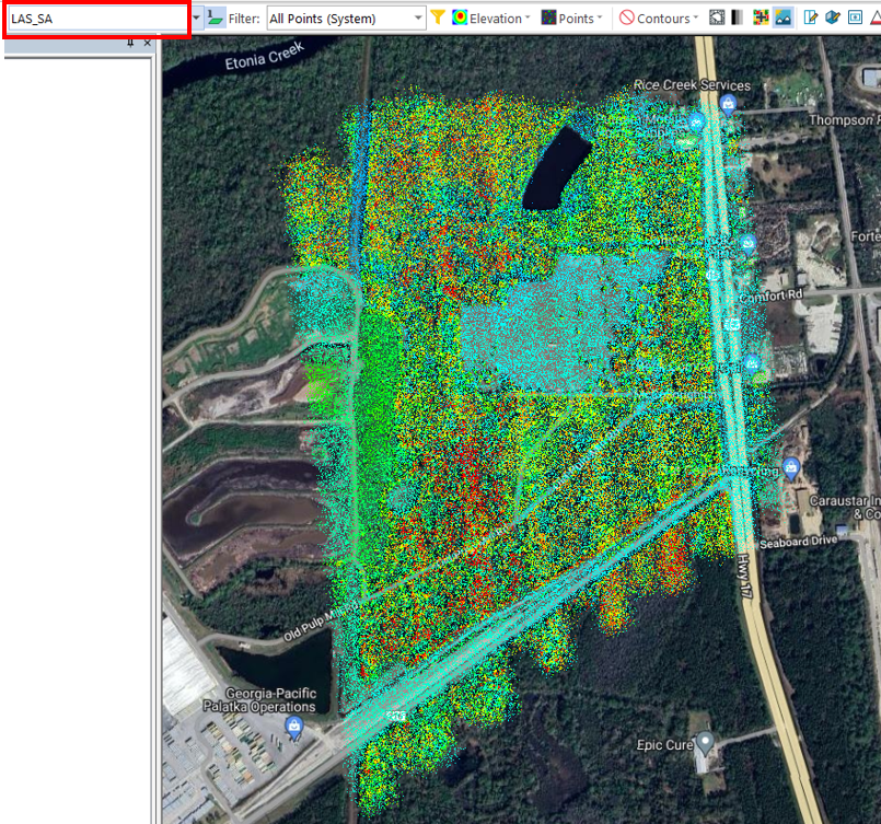
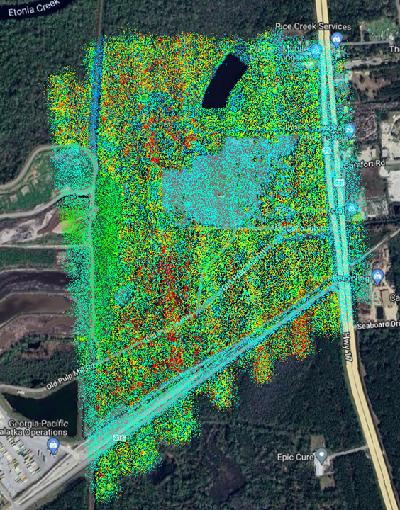
Strip Align will create a new LAS, in my case it is called “LAS_SA”. This new LAS has all the misalignments corrected. Example:
5. Control Points
In this section, we will add check points and compare them to our point cloud. At this step we want first know what the accuracy of our point cloud compared to the check points. After that, we will analyze if there is any bias (constant offset in all the point cloud). If there is, we will remove it and create a final QC accuracy report.
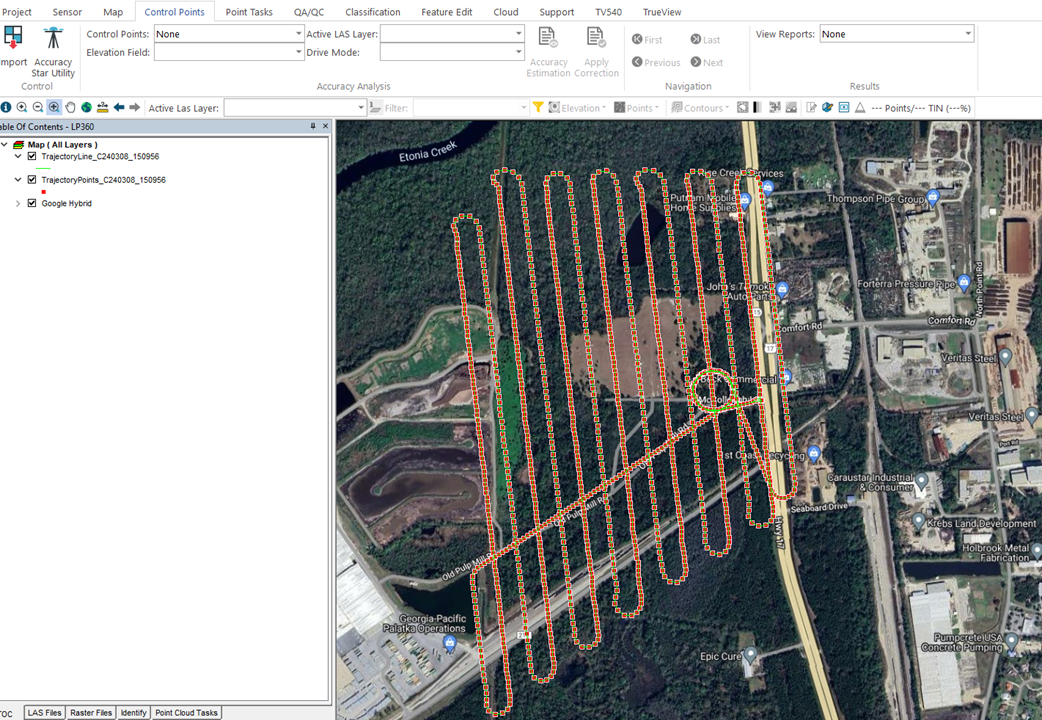
1- Go to Control Point ribbon
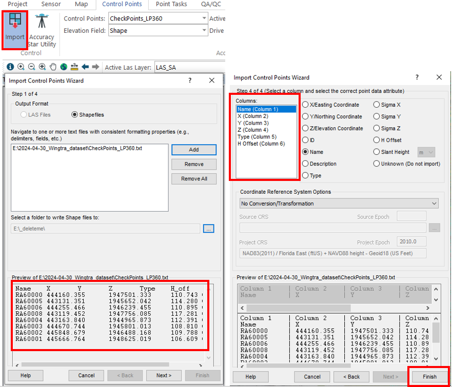
2- Select “Import”
3- Import the control points in .csv or .txt format
Tip: before importing the control points, make sure to add the control point type and height offset from the ground. Summary:
– Vertical check point –> VK (autodetected only in vertical)
– Full check point –> FK (autodetected only in vertical)
– Check board –> CB (autodetected in horizontal and vertical)
– Accuracy Star –> AS (autodetected in horizontal and vertical)
– Height offset –> 0 if the points are in the ground
4- Example of a control point file format
Name	X	Y	Z	Type	H_off
RA60000	444160.355	1947501.333	110.743	CB	0
RA60005	443131.351	1945652.042	114.280	CB	0
RA60006	444255.466	1946239.455	110.895	CB	0
RA60008	443119.452	1947756.085	117.281	CB	0
RA60004	443163.840	1944965.873	112.391	CB	0
RA60003	444670.744	1945801.013	108.810	CB	0
RA60002	445848.679	1946488.168	109.788	CB	0
RA60001	445666.764	1948625.019	106.609	CB	0
5- Make sure to have selected the Strip Align LAS (LAS_SA). It should appear as “Active LAS Layer”
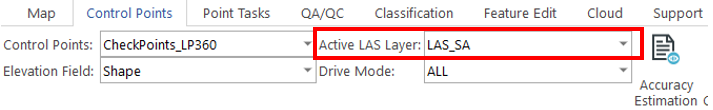
6- Press “Accuracy Estimation” –> Press “Auto Find”
Tip: If you are using Checker Boards go to –> Settings… –> Select the Target size
7- Control Point report will be populated, with statistics for each control point.
Tip: remember the control point type, only CB and AS will have the automatic measurement in horizontal and vertical. The rest of types will automatically measure only in vertical.
The automatic detection of Checker Boards and Accuracy Star requires the license “3D accuracy“
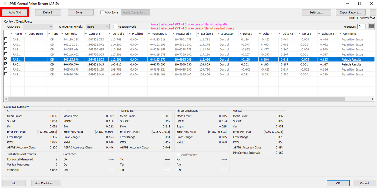
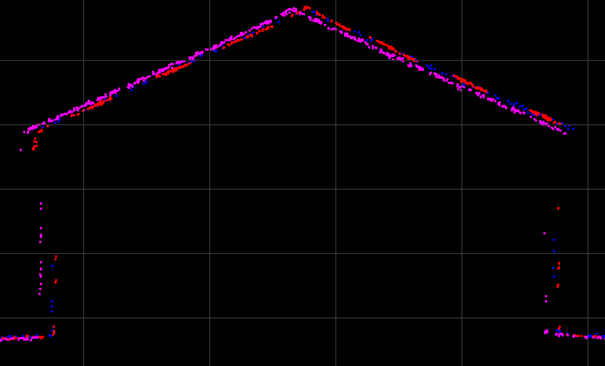
8- The report will show the difference between each point to the point cloud. If it has an automatic detection, will also add a comment on how reliable the measurement was.
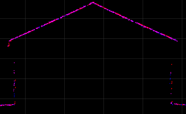
9- If we detect a bias, like the example, we will press “Solve…” to fix it.
10- A new layer called “LAS Layer_1” will be created with the debias point cloud. I recommend calling this layer “LAS_SA_debias”.
Tip: the name used is a combination of the layer type “LAS”, and the corrections applied. In this case first strip align “SA” and later remove any possible bias “debias”.
11- Optional, select the new debias layer (LAS_SA_debias) and measure again the check points. This will create a final report with the accuracy of the flight. You can export the report with the “Export Report…” button.
6. Smoothing
In this section we will apply smoothing algorithm to our LAS, this will reduce the point cloud noise envelope or the thickness of the point cloud. This algorithm works well for manmade structures, flat areas or regular surfaces.
1- Go to Point Cloud Tasks tab
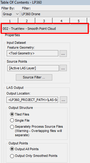
2- Select from the list “002 – TrueView – Smooth Point Cloud“
If the PCT isn’t in the list, you can create it –> Add –> Smoothing, Point Cloud
3- Configure the PCT (no need to changed any setting if “002 – TrueView – Smooth Point Cloud” is selected)
Output Location –> Select a folder
Tiles Files: checked
Output all points –> checked
4- Press “Apply” in the PCT if any setting was changed
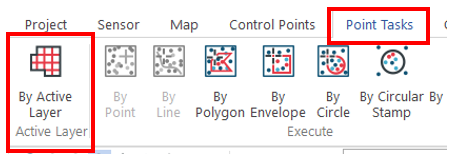
5- Perform the PCT –>Point Tasks ribbon –> By Active Layer
Once the PCT finish there will be a new LAS layer called “LAS Layer_1”, we will rename the layer to “LAS_SA_debias_RGB_SM”, SM comes from smoothing.
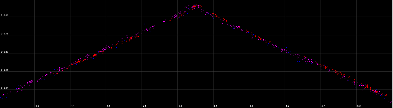
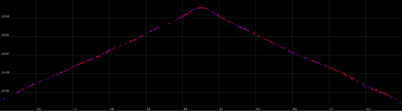
We reduced the point cloud noise envelope from 0.2ft to 0.05ft, or from 8cm to 2cm.
7. Point Cloud colorization (optional)
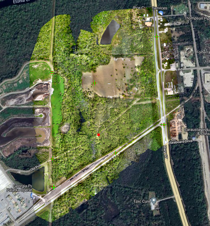
Only required if the point cloud is not colorized in your UAV LiDAR software. The colour source can be from a camera integrated with the LiDAR sensor or from a difference source. In this section we will see how to colorize the point cloud from an orthophoto.
7.1. Import an orthophoto
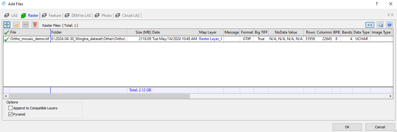
1- Go to Project ribbon –> Add Files
2- Go to Raster tab –> Press “+” –> Add an orthophoto
Tip: the orthophoto needs to be in the same CRS as the project. If it is not, you will need to reproject it before performing the following steps.
7.2. Color by Image
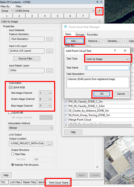
1- Go to Point Cloud task tab –> PCT Manager Dialog![]() –> Add –> Task Type: Color by Image –> Task Name: Color by Image
–> Add –> Task Type: Color by Image –> Task Name: Color by Image
2- Select the PCT
3- Configure the PCT.
Input Raster Layer: Ortho (the orthophoto we added)
LiDAR RGB: Checked
Red Image Channel: 1
Green Image Channel: 2
Blue Image Channel: 3
Interpolation Method: Bilinear
Las Output: Select a folder to save the new LAS
Check Maintain File Structure
4- Press “Apply” in the “Color by Image” PCT
5- Perform the PCT –>Point Task tab –> By Active Layer
Once the PCT finish there will be a new LAS layer called “LAS Layer_1”, we will rename the layer to “LAS_SA_debias_RGB”, RGB comes from the colorization. This LAS is colorized, we can view it by “rgb”.
8. Export final LAS
In this section we will export our final point cloud in a single LAS file.
8.1. Create Area of Interest
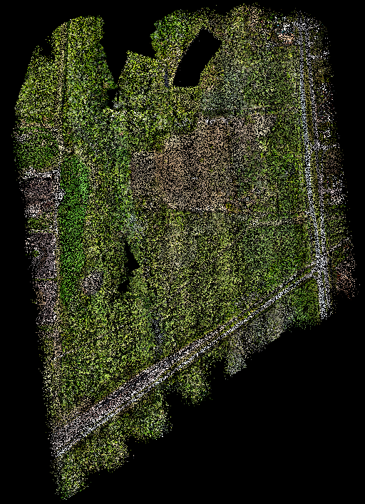
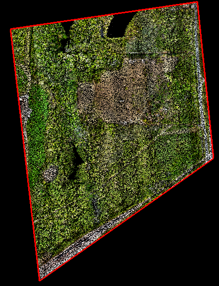
We will crop the point cloud to limit it only to the area of interest, this means cutting the corners of the flight.
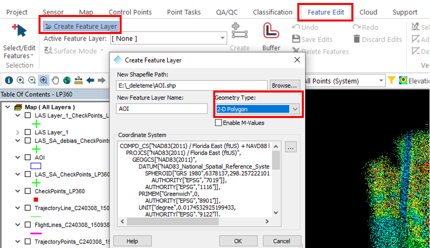
1- Go to Feature Edit ribbon –> Create Feature Layer
2- Press browse… –> Select a folder to save the layer –> Give a name to the layer –> Geometry Type: 2D Polygon –> OK
3- Press “Create Feature” –> Create a polygon –> Right click “Finish Edit”
4- Press “Save Edits”
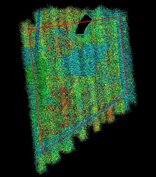
We created a polygon that contains our area of interest. In the next step we will export only the points contained inside the AOI.
8.2. Export final point cloud
1- Make sure to set “Active LAS Layer” the latest LAS layer, in the example – “LAS_SA_debias_RGB_SM”
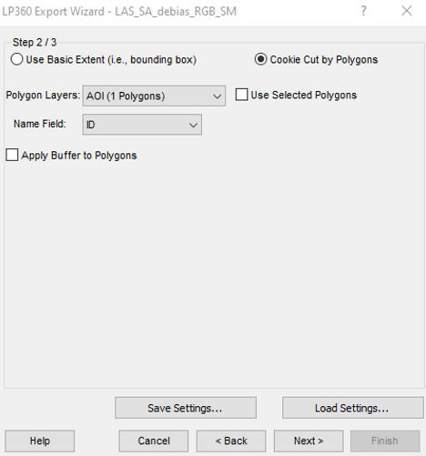
2- Go to Project tab –> Export Wizard –> Press Next
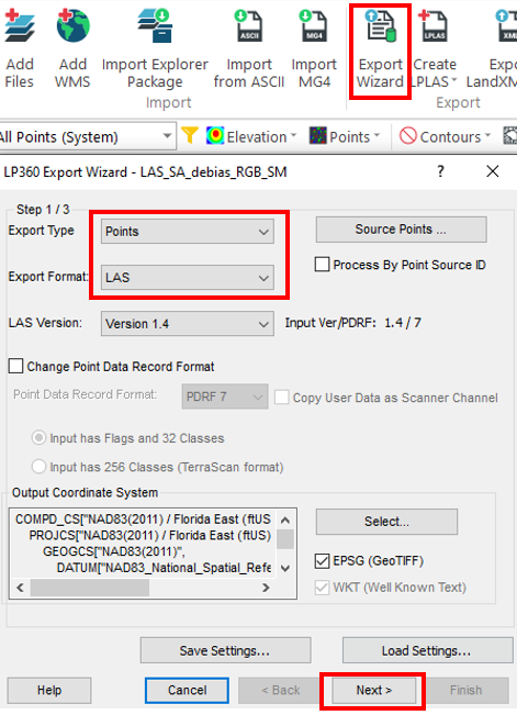
3- Select “Cookie Cut by Polygons” –> Select “AOI” Polygon –> Press Next
4- Select a export path folder location
Tip: always save each final deliverable in a new folder
5- Press Finish
We have generated our final LAS. If we go to the export folder we will see a single LAS file.
This LAS file contains all the corrections we applied during in the article
